2.2.4.2. Wilks-quantile computation
The Wilks quantile computation is an empirical estimation, based on order statistic which allows to get an estimation on the requested quantile, with a given confidence level \(\beta\), independently of the nature of the law, and most of the time, requesting less estimations than a classical estimation. Going back to the empirical way discussed in Empirical computation: it consists, for a 95% quantile, in running 100 computations, ordering the obtained values and taking the one at either the 95-Th or 96-Th position (see the discussion on how to choose k in Empirical computation). This can be repeated several times and will result in a distribution of all the obtained quantile values peaking at the theoretical value, with a standard deviation depending on the number of computations made. As it peaks on the theoretical value, 50% of the estimation are larger than the theoretical value while the other 50% are smaller (see Figure 2.21 for illustration purpose).
Wilks computation on the other hand request not only a probability value but also a confidence level. The quantile \(x_p^\beta\) represents the \(x_p\) quantile given the \(p\) probability but this time, the value is provided with a \(\beta\)% confidence level, meaning that \(\beta\)% of the obtain value is larger than the theoretical quantile. This is a way to be conservative and to be able to quantify how conservative one wants to be. To do this, the size of the sample must follow a necessary condition:
This is the smallest sample size to get an estimation, and, in most cases, the accuracy reached (for a given sample size) is better than the one achieved with the simpler solution provided above. It is also possible to increase the sample size to get a better description of the quantile estimation.
Figure 2.21 Illustration of the results of 100000 quantile determinations, applied to a reduced centered
gaussian distribution, comparing the usual and Wilks methods. The number of points in the
reduced centered gaussian distribution is varied, as well as the confidence level.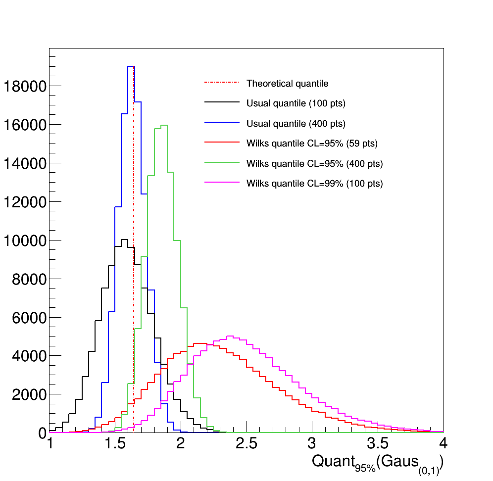
Figure 2.21 shows a simple case: the estimation of the value of the 95% quantile of a centered-reduced normal distribution. The theoretical value (red dashed line) is compared to the results of 100000 empirical estimation, following the simple recipe (black and blue curves) or the Wilks method (red, green and magenta curves). Several conclusions can be drawn:
The simpler quantile estimation average is slightly biased with respect to the theoretical value. This is due to the choice of k, discussed in Empirical computation which can lead to under or over estimation of the quantile value. The bias becomes smaller with the increasing sample size.
The standard deviation of the distributions (whatever method is considered) is becoming smaller with the increasing sample size.
When using the Wilks method, the fraction of event below the theoretical value is becoming smaller with the increasing confidence level.