3.6.3.4. Random mode

In order to have randomly distributed values over the interval, the example’s code needs further modifications.

To produce a random sampling, the attributes representing the factors must belong to the TStochasticAttribute family (cf. Introducing the TStochasticAttribute classes). We thus need to modify the “step 1” of example of Construction of a simple OAT design-of-experiments to:

    TDataServer *tds = new TDataServer("tdsoat","Data server for simple OAT design");

    // step 1
    tds->addAttribute(new TUniformDistribution("x1", -5.0, 5.0));
    tds->addAttribute(new TNormalDistribution("x2", 11.0, 1.0));

Tip

There is no a priori relationship between the distribution of the attribute and the nominal value and range of the factor it represents. However, a good practice is to insure that the probability density over the whole factor’s range is never null.

The “step 2” of the example of Construction of a simple OAT design-of-experiments does not need to be modified. The “step 3”, on the other hand, becomes:

    // step 3
    TOATDesign *oatSampler = new TOATDesign(tds, "lhs", 1000);

By choosing the “lhs” mode, we ask for a random sampling over the range of the factor (defined in “step 4”). Here, we also ask for 1000[1] modifications of each factor.

The rest of the script remains unchanged. We modify the “//display” section in order to visualise histograms of the sampling, instead of a long list of numbers:

    TCanvas c("can","can",10,32,1200,600);
    // display
    TPad *apad = new TPad("apad","apad",0, 0.03, 1, 1);
    apad->Draw();
    apad->Divide(2,1);
    apad->cd(1);
    tds->draw("x1","__modified_att__ == 1");
    apad->cd(2);
    tds->draw("x2","__modified_att__ == 2");

Tip

The two calls to draw are an illustration of the use of the “__modified_att__” attribute. Here, it allows to filter out the data, by keeping only the experiments where the interesting factor is modified.

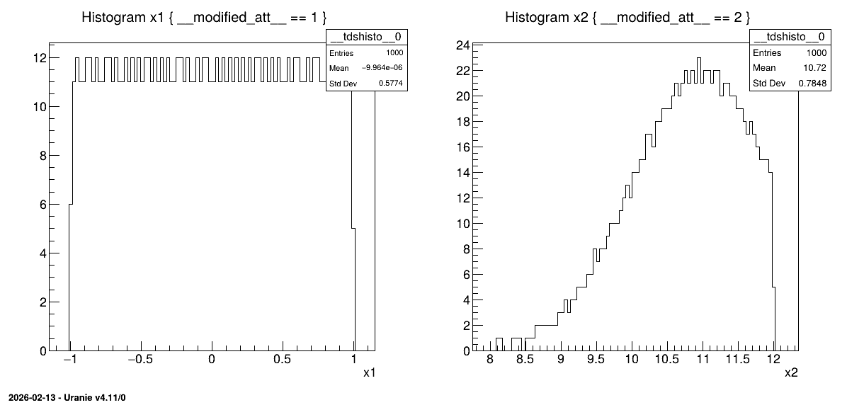
The resulting histograms are shown in figure Figure 3.15. The left histogram shows the distribution of data for the “x1” attribute (uniform distribution) and the right, for the “x2” attribute (gaussian distribution). The latter shows how the gaussian distribution is truncated by the choice of the nominal value and the range (the complete code can be found in Macro “samplingOATRandom.C”).