3.1. Introduction
The Sampler module is used to produce design-of-experiments knowing the expected behaviour of the input variables for the problem under consideration. The framework of our approach can be illustrated in the following schematic view:
Figure 3.1 Schematic view of the input/output relation through a code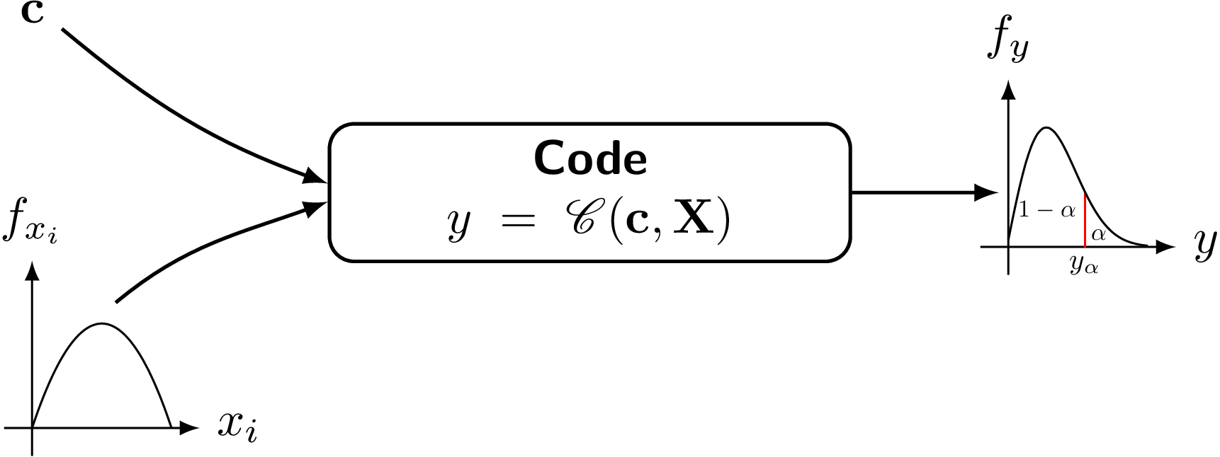
We will denote as \(\mathcal{C}\) the studied computational code which, generally, has two types of inputs:
The constant parameters which are gathered in the vector \(\mathbf{c} \in {\rm I\!R}^{n_C}\). They represent constants.
The uncertain parameters which are gathered in the vector \(\mathbf{X} \in {\rm I\!R}^{n_X}\)
It shall be noticed that these parameters are supposed to be uncertain either because of a lack of knowledge on their actual value or because of their intrinsic random nature.
The result of the code \(\mathcal{C}\) for a given set of parameters \((\mathbf{c},\mathbf{X})\) gives the vector \( y \in {\rm I\!R}^{n_Y} = \mathcal{C} ( \mathbf{c}, \mathbf{X})\) which contains all the output variables of the analysis.
Different methods exist to obtain a design-of-experiments from uncertain parameters which can be classified into two categories:
stochastic methods (see The Stochastic methods). These methods consist in using a random number generator to produce new samples. This is also called Monte-Carlo.
deterministic methods (see QMC method). Two distinct calls with the same parameters will always give the same point in a design-of-experiments. Some of these methods (those discussed below) are sequences which are sometimes called quasi-Monte Carlo (qMC).