3.2.3.1. Introduction
Considering the definition of a LHS sampling, introduced in Introduction, it is clear that permutating a coordinate of two different points, will create a new sampling. If one looks at the x-coordinate (corresponding to a normal distribution) in Figure 3.2, one could put the point in the second equi-probable range, in the sixth one, and move the point which was in the sixth equi-probable range into the second one, without changing the y-coordinate. The results of this permutation is a new sampling with the interesting property of remaining a LHS sampling. A follow-up question can then be: what is the difference between these two samplings, and would there be any reason to try many permutations ?
This is a very brief introduction to a dedicated field of research: the optimisation of a design-of-experiments with respect to the goals of the ongoing analysis. In Uranie, a new kind of LHS sampling has been recently introduced, called maximin LHS, whose purpose is to maximise the minimal distance between two points. The distance under consideration is the mindist criterion: let \(D=[\mathbf{x}_1, \cdots,\mathbf{x}_N] \subset [0,1]^{d}\) be a design-of-experiments with \(N\) points. The mindist criterion is written as:
where \(||.||_2\) is the euclidian norm. The designs which maximise the mindist criterion are referred to as maximin LHS, but generally speaking, a design with a large value of the mindist criterion is referred to as maximin LHS as well. It has been observed that the best designs in terms of maximising (Equation 3.4) can be constructed by minimising its \(L^{p}\) regularisation instead. It is written as
Figure 3.4 shows, on the left, an example of a LHS when considering a problem with two uniform distributions between 0 and 1 but also, on the right, its transformation through the maximin optimisation. The mindist criterion is displayed on top for comparison purpose.
Figure 3.4 Transformation of a classical LHS (left) to its corresponding maximin LHS (right) when
considering a problem with two uniform distributions between 0 and 1.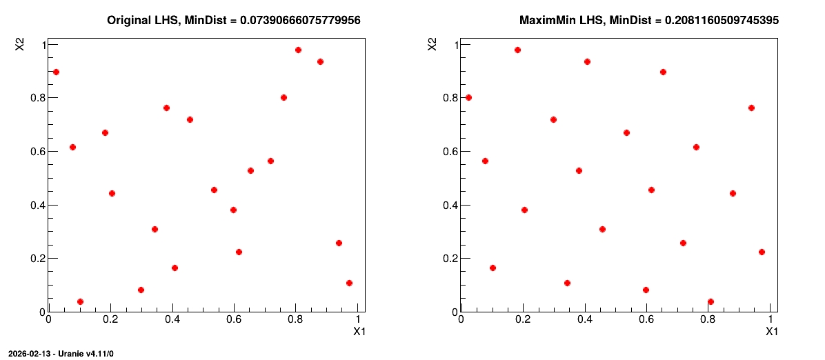
From a theoretical perspective, using a maximin LHS to build a Gaussian process (GP) emulator can reduce the predictive variance when the distribution of the GP is exactly known. However, it is not often the case in real applications where both the variance and the range parameters of the GP are actually estimated from a set of learning simulations run over the maximin LHS. Unfortunately, the locations of maximin LHS are far from each other, which is not a good feature to estimate these parameters with precision. That is why maximin LHS should be used with care. Relevant discussions dealing with this issue can be found in [PM12].