3.2.1. Introduction

In these methods the knowledge (or mis-knowledge) of the model is encoded in the choice of probability law used to describe the inputs \(x_{i}\), for \(i \, \in \, [0,\, n_X]\). These laws are usually defined by:

• a range that describes the possible values of \(x_{i}\)

• the nature of the law, which has to be taken in the list of pre-defined laws already presented in The probability distributions

A choice has frequently to be made between two implemented methods of drawing:

SRS (Simple Random Sampling):

This method consists in independently generating the samples for each parameter following its own probability density function. The obtained parameter variance is rather high, meaning that the precision of the estimation is poor leading to a need for many repetitions in order to reach a satisfactory precision. An example of this sampling when having two independent random variables (uniform and normal one) is shown in Figure 3.3-left. In order to get this drawing, the variable are normalised from 0 to 1 and a random drawing is performed in this range. The obtained value is computed calling the inverse CDF function corresponding to the law under study (that one can see from Figure 2.2 until Figure 2.18).

LHS (Latin Hypercube Sampling):

this method [MBC00] consists in partitioning the interval of each parameter so as to obtain segments of equal probabilities, and afterwards in selecting, for each segment, a value representing this segment. An example of this sampling when having two independent random variables (uniform and normal one) is shown in Figure 3.3-right. In order to get this drawing, the variable are normalised from 0 to 1 and this range is split into the requested number of points for the design-of-experiments. Thanks to this, a grid is prepared, assuring equi-probability in every sub-space. Finally, a random drawing is performed in every sub-range. The obtained value is computed calling the inverse CDF function corresponding to the law under study (that one can see from Figure 2.2 until Figure 2.18).

The first method is fine when the computation time of a simulation is “satisfactory”. As a matter of fact, it has the advantage of being easy to implement and to explain; and it produces estimators with good properties not only for the mean value but also for the variance. Naturally, it is necessary to be careful in the sense to be given to the term “satisfactory”. If the objective is to obtain quantiles for extreme probability values \(\alpha\) (i.e. \(\alpha\) = 0.99999 for instance), even for a very low computation time, the size of the sample would be too large for this method to be used. When a computation time becomes important, the LHS sampling method is preferable to get robust results even with small-size samples (i.e. \(N_{\rm calc}\) = 50 to 200) [HD02]. On the other hand, it is rather trivial to double the size of an existing SRS sampling, as no extra caution has to be taken apart from the random seed.

In Figure 3.2, we present two samples of size \(N_{\rm calc}\) = 8 coming from these two sampling methods for two random variables \(U_1\) according to a gaussian law, and \(U_2\) a uniform law. To make the comparison easier, we have represented on both figures the partition grid of equiprobable segments of the LHS method, keeping in mind that it is not used by the SRS method. These figures clearly show that for LHS method each variable is represented on the whole domain of variation, which is not the case for the SRS method. This latter gives samples that are concentrated around the mean vector; the extremes of distribution being, by definition, rare.

Concerning the LHS method (right figure), once a point has been chosen in a segment of the first variable \(U_1\), no other point of this segment will be picked up later, which is hinted by the vertical red bar. It is the same thing for all other variables, and this process is repeated until the \(N_{\rm calc}\) points are obtained. This elementary principle will ensure that the domain of variation of each variable is totally covered in a homogeneous way. On the other hand, it is absolutely not possible to remove or add points to a LHS sampling without having to regenerate it completely. A more realistic picture is draw in Figure 3.3 with the same laws, both for SRS on the left and LHS on the right which clearly shows the difference between both methods when considering one-dimensional distribution.

Figure 3.2 Comparison of the two sampling methods SRS (left) and LHS (right) with samples of size 8.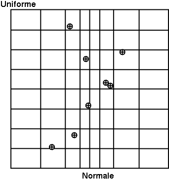

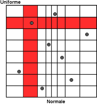
Figure 3.3 Comparison of deterministic design-of-experiments obtained using either SRS (left) or LHS (right) algorithm, when having two independent random variables (uniform and normal one)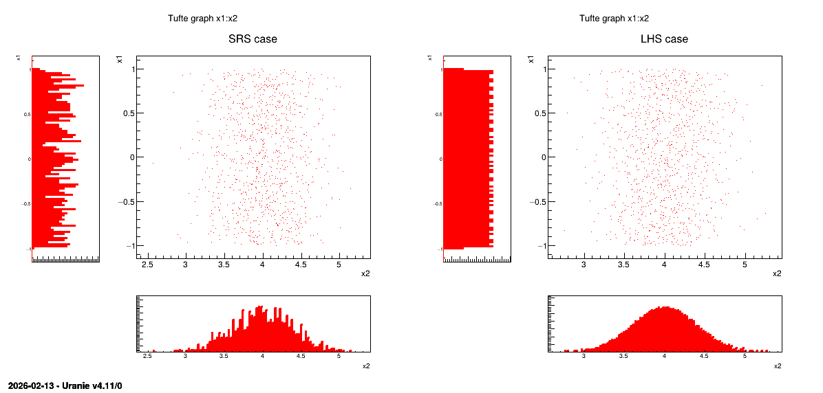

There are two different sub-categories of LHS design-of-experiments discussed here and whose goal might slightly differs from the main LHS design discussed above:

• the maximin LHS: this category is the result of an optimisation whose purpose is to maximise the minimal distance between any sets of two locations. This is discussed later-on in The maximin LHS.

• the constrained LHS: this category is defined by the fact that someone wants to have a design-of-experiments fulfilling all properties of a Latin Hypercube Design but adding one or more constraints on the input space definition (generally inducing correlation between varibles). This is also further discussed in The constrained LHS.

Once the nature of the law is chosen, along with a variation range, for all inputs \(x_{i}\), the correlation between these variables has to be taken into account. It is doable by defining a correlation coefficient but the way it is treated from one sampler to the other is tricky and is further discussed in the next section.