2.1.1.19. Composing law

It is possible to imagine a new law, hereafter called composed law, by combining different pre-existing laws in order to model a wanted behaviour. This law would be defined with \(N\) pre-existing laws whose densities are noted \(\lbrace f_j\rbrace_{1\leq j \leq N }\), along with their relative weights \(\lbrace \omega_j\rbrace_{1\leq j \leq N } \in (\mathbb{R}^{+})^{N}\) and the resulting density is then written as

\[f(x) = \sum_{j=1}^{N} \omega_j f_j(x)\]

The mean value of this newly generated law can be expressed, assuming that all pre-existing laws have a finite and defined expectation denoted \(\lbrace \mu_j\rbrace_{1\leq j\leq N }\), as \(\mu = \sum_{j=1}^{N}\frac{\omega_j \mu_j}{S}\)
where the sum of all weights is \(S = \sum_{j=1}^{N} \omega_j\). As for the mean value, the variance of this newly generated law can be expressed, assuming that all pre-existing laws have a finite and defined expectation and variance, as done below in a very generic way.

\[\begin{split}\begin{split} {\rm Var}_f & = \mathbb{E}_f(x^2) - (\mathbb{E}_f(x))^2 \nonumber \\ & = \int x^2 f(x) dx - \bigg(\int xf(x)dx\bigg)^2, \;\, {\rm with} \;\, f(x) = \sum_{j=1}^{N} \omega_j f_j(x) \;\, \rm{where} \;\, \lbrace \omega_j\rbrace_{1\leq j \leq N} \in (\mathbb{R}^{+})^N \nonumber \\ & = \int \sum^{N}_{j=1} x^2 \frac{\omega_jf_j(x)}{S} dx - \bigg(\int \sum^{N}_{j=1} x \frac{\omega_jf_j(x)}{S} dx\bigg)^2, \;\, \rm{where} \;\, S = \sum_{j=1}^N \omega_j \nonumber \\ & = \frac{1}{S} \sum^{N}_{j=1} \omega_j \underbrace{\int x^2 f_j(x) dx}_{{\rm Var}_{f_j}(x) + (\mathbb{E}_{f_j}(x))^2 } - \frac{1}{S^2}\bigg(\sum^{N}_{j=1} \omega_j\underbrace{\int x f_j(x) dx}_{\mathbb{E}_{f_j}(x)}\bigg)^2\nonumber \\ & = \frac{1}{S} \sum^{N}_{j=1} \omega_j (\sigma^2_j + \mu_j^2) - \frac{1}{S^2} \bigg(\sum^{N}_{j=1} \delta_j\bigg)^2,\;\, {\rm where} \;\, \delta_j = \omega_j \mu_j \;\, \forall j \in [1,N] \nonumber \\ & = \frac{1}{S} \sum^{N}_{j=1} \omega_j\sigma^2_j + \sum^{N}_{j=1} \frac{\delta_j^2}{S \omega_j} - \frac{1}{S^2} \bigg[ \sum^{N}_{j=1} \delta^2_j + 2\sum_{1\leq i < j \leq N} \delta_i\delta_j \bigg]\nonumber \\ & = \frac{1}{S} \sum^{N}_{j=1} \omega_j\sigma^2_j + \sum^{N}_{j=1} \frac{S-\omega_j}{S^2 \omega_j} \delta_j^2 - \frac{2}{S^2} \sum_{1\leq i < j \leq N} \delta_i\delta_j. \end{split}\end{split}\]

In the case of unweighted composition, this can be written as \(\displaystyle{\rm Var}_f = \frac{1}{N}\sum^{N}_{j=1} \sigma^2_j + \frac{N-1}{N^2} \sum^{N}_{j=1} \mu_j^2 - \frac{2}{N^2} \sum_{1\leq i < j \leq N} \mu_i\mu_j\) .

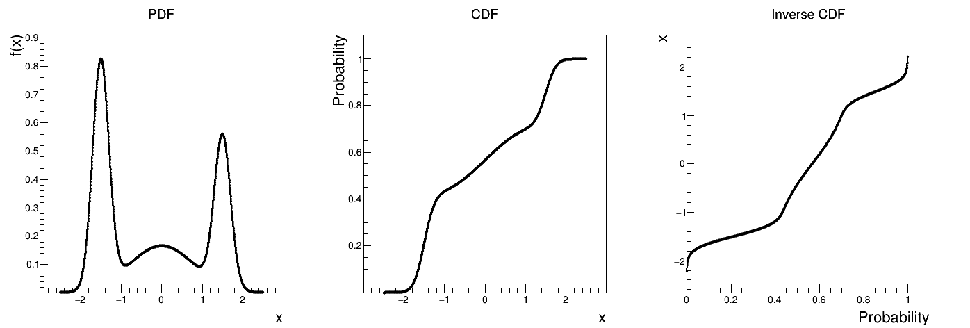
Figure 2.20 shows the PDF, CDF and inverse CDF generated for different sets of parameters.

Figure 2.20 Example of PDF, CDF and inverse CDF for a composed distribution made out of three normal distributions with respective weights.