2.1.1. The probability distributions
There are several already-implemented statistical laws in Uranie, that can be called marginal laws as well, used to described the behaviour of a chosen input variable. They are usually characterised by two functions which are intrinsically connected: the PDF (probability density function) and CDF (cumulative distribution function). One can recap briefly the definition of these two functions for every random variable \(X : \Omega \rightarrow \rm I\!R\) :
PDF: if the random variable X has a density \(f_X\), where \(f_X\) is a non-negative Lebesgue-integrable function, then
CDF: the function \(F_{X} : {\rm I\!R} \rightarrow [0,1]\), given by
For some of the distributions discussed later on, the parameters provided to define them are not
limiting the range of their PDF and CDF: these distributions are said to be infinite-based ones.
It is however possible to set boundaries in order to truncate the span of their possible values.
One can indeed define an lower bound \(L\) and or an upper bound \(U\) so that the resulting distribution
range is not infinite anymore but only in \([L, U]\). This truncation step affects both the PDF and CDF:
once the boundaries are set, the CDF of these two values are computed to obtain \(P_{L}\) (the
probability to be lower than the lower edge) and \(P_{U}\) (the probability to be lower than the upper
edge). Two new functions, the truncated PDF \(f_{X}^{[L,U]}\) and the truncated CDF \(F_{X}^{[L,U]}\)
are simply defined as
These steps to produce a truncate distribution are represented in Figure 2.1 where the original distribution is shown on the left along with the definition of \(L\) (the blue shaded part) and \(U\) (the green shaded part). The right part of the plot is the resulting truncated PDF.
Figure 2.1 Principle of the truncated PDF generation (right-hand side) from the orginal one (left-hand side).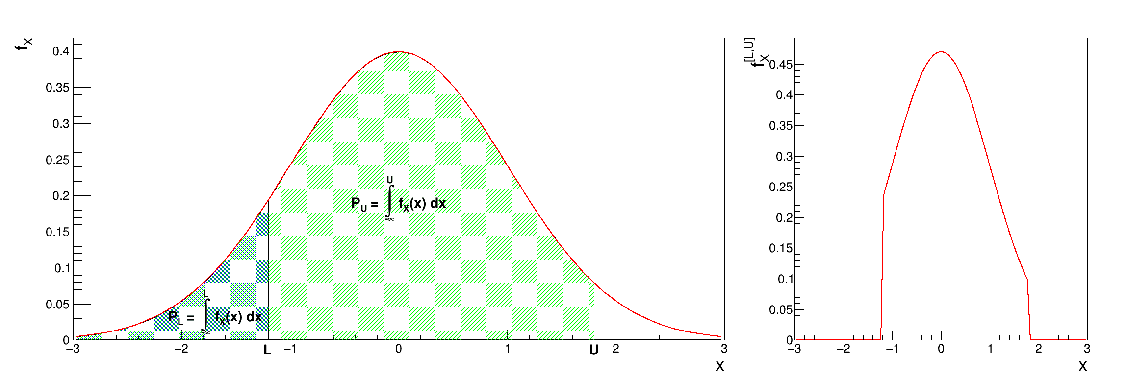
It is possible to combine different probability law, as a sum of weighted contributions, in order to create a new law. This approach, which is further discussed and illustrated in Composing law, leads to a new probability density function that would look like
These distributions can be used to model the behaviour of variables, depending on chosen hypothesis, probability density function being used as a reference more oftenly by physicist, whereas statistical experts will generally use the cumulative distribution function [App13].
Table 2.1 gathers the list of implemented statistical laws, along with the list of parameters used to define them. For every possible law, a figure is displaying the PDF, CDF and inverse CDF for different sets of parameters (the equation of the corresponding PDF is reminded as well on every figure). The inverse CDF is basically the CDF whose x and y-axis are inverted (it is convenient to keep in mind what it looks like, as it will be used to produce design-of-experiments, later-on).
Law |
Class Uranie |
Parameter 1 |
Parameter 2 |
Parameter 3 |
Parameter 4 |
|---|---|---|---|---|---|
Uniform |
Min |
Max |
|||
Log-Uniform |
Min |
Max |
|||
Triangular |
Min |
Max |
Mode |
||
Log-Triangular |
Min |
Max |
Mode |
||
Normal (Gauss) |
Mean (\(\mu\)) |
Sigma (\(\sigma\)) |
|||
Log-Normal |
Mean (\(M\)) |
Error factor (\(E_f\)) |
Min |
||
Trapezium |
Min |
Max |
Low |
Up |
|
UniformByParts |
Min |
Max |
Median |
||
Exponential |
Rate (\(\lambda\)) |
Min |
|||
Cauchy |
Scale (\(\gamma\)) |
Median |
|||
GumbelMax |
Mode (\(\mu\)) |
Scale (\(\beta\)) |
|||
Weibull |
Scale (\(\lambda\)) |
Shape (\(k\)) |
Min |
||
Beta |
alpha (\(\alpha\)) |
beta (\(\beta\)) |
Min |
Max |
|
GenPareto |
Location (\(\mu\)) |
Scale (\(\sigma\)) |
Shape (\(\xi\)) |
||
Gamma |
Shape (\(\alpha\)) |
Scale (\(\beta\)) |
Location (\(\xi\)) |
||
InvGamma |
Shape (\(\alpha\)) |
Scale (\(\beta\)) |
Location (\(\xi\)) |
||
Student |
DoF (\(k\)) |
||||
GeneralizedNormal |
Location (\(\mu\)) |
Scale (\(\alpha\)) |
Shape (\(\beta\)) |
- 2.1.1.1. Uniform Law
- 2.1.1.2. Log Uniform Law
- 2.1.1.3. Triangular Law
- 2.1.1.4. LogTriangular Law
- 2.1.1.5. Normal law
- 2.1.1.6. LogNormal law
- 2.1.1.7. Trapezium law
- 2.1.1.8. UniformByParts law
- 2.1.1.9. Exponential law
- 2.1.1.10. Cauchy law
- 2.1.1.11. GumbelMax law
- 2.1.1.12. Weibull law
- 2.1.1.13. Beta law
- 2.1.1.14. GenPareto law
- 2.1.1.15. Gamma law
- 2.1.1.16. InvGamma law
- 2.1.1.17. Student Law
- 2.1.1.18. Generalized normal law
- 2.1.1.19. Composing law