13.3.16. Macro “dataserverDrawPPPlot.py”

13.3.16.1. Objective

This macro is an example of how to produce PP-plot for a certain number of randomly-drawn samples, providing the correct parameter values along with modified versions to illustrate the impact.

13.3.16.2. Macro Uranie

"""
Example of PP plot
"""
from URANIE import DataServer, Sampler
import ROOT

# Create a TDS with 8 kind of distributions
p1 = 1.3
p2 = 4.5
p3 = 0.9
p4 = 4.4  # Fixed values for parameters

tds0 = DataServer.TDataServer()
tds0.addAttribute(DataServer.TNormalDistribution("norm", p1, p2))
tds0.addAttribute(DataServer.TLogNormalDistribution("logn", p1, p2))
tds0.addAttribute(DataServer.TUniformDistribution("unif", p1, p2))
tds0.addAttribute(DataServer.TExponentialDistribution("expo", p1, p2))
tds0.addAttribute(DataServer.TGammaDistribution("gamm", p1, p2, p3))
tds0.addAttribute(DataServer.TBetaDistribution("beta", p1, p2, p3, p4))
tds0.addAttribute(DataServer.TWeibullDistribution("weib", p1, p2, p3))
tds0.addAttribute(DataServer.TGumbelMaxDistribution("gumb", p1, p2))

# Create the sample
fsamp = Sampler.TBasicSampling(tds0, "lhs", 200)
fsamp.generateSample()

# Define number of laws, their name and numbers of parameters
nLaws = 8
# number of parameters to put in () for the corresponding law
laws = ["normal", "lognormal", "uniform", "gamma",
        "weibull", "beta", "exponential", "gumbelmax"]
npar = [2, 2, 2, 3, 3, 4, 2, 2]

# Create the canvas
c = ROOT.TCanvas("c1", "", 800, 1000)
# Create the 8 pads
apad = ROOT.TPad("apad", "apad", 0, 0.03, 1, 1)
apad.Draw()
apad.cd()
apad.Divide(2, 4)

# Number of points to compare theoretical and empirical values
nS = 1000
mod = 0.8  # Factor used to artificially change the parameter values

Par = lambda i, n, p, mod: ","+str(p*mod) if n >= i else ""
opt = ""  # option of the drawPPPlot method
for i in range(nLaws):

    # Clean sstr
    test = ""
    # Add nominal configuration
    test += laws[i] + "(" + str(p1) + "," + str(p2) + Par(3, npar[i], p3, 1) \
        + str(p2) + Par(4, npar[i], p4, 1) + ")"
    # Changing par1
    test += ":" + laws[i] + "(" + str(p1*mod) + "," + str(p2) \
        + Par(3, npar[i], p3, 1) + str(p2) + Par(4, npar[i], p4, 1) + ")"
    # Changing par2
    test += ":" + laws[i] + "(" + str(p1) + "," + str(p2*mod) \
        + Par(3, npar[i], p3, 1) + str(p2) + Par(4, npar[i], p4, 1) + ")"
    # Changing par3
    if npar[i] >= 3:
        test += ":" + laws[i] + "(" + str(p1) + "," + str(p2) \
            + Par(3, npar[i], p3, mod) + str(p2) + Par(4, npar[i], p4, 1) + ")"
    # Changing par4
    if npar[i] >= 4:
        test += ":" + laws[i] + "(" + str(p1) + "," + str(p2) \
            + Par(3, npar[i], p3, 1) + str(p2) + Par(4, npar[i], p4, mod) + ")"

    apad.cd(i+1)
    # Produce the plot
    tds0.drawPPPlot(laws[i][:4], test, nS, opt)

The macro is based on the one discussed in Macro “dataserverDrawQQPlot.py”. The only difference is this line

    tds0.drawPPPlot(laws[i][:4], test, nS, opt)

The call of the drawing method above can be resume, for the first case, like this:

tds0.drawPPPlot( "norm", "normal(1.3,4.5):normal(1.04,4.5):normal(1.3,3.6)", nS)

The first field is the attribute to be tested, while the second one provides the three hypothesis with which our attribute under investigation will be compared. The third argument is the number of steps to be computed for probabilities.

The result of this macro is shown below.

13.3.16.3. Graph

Figure 13.8 Graph of the macro 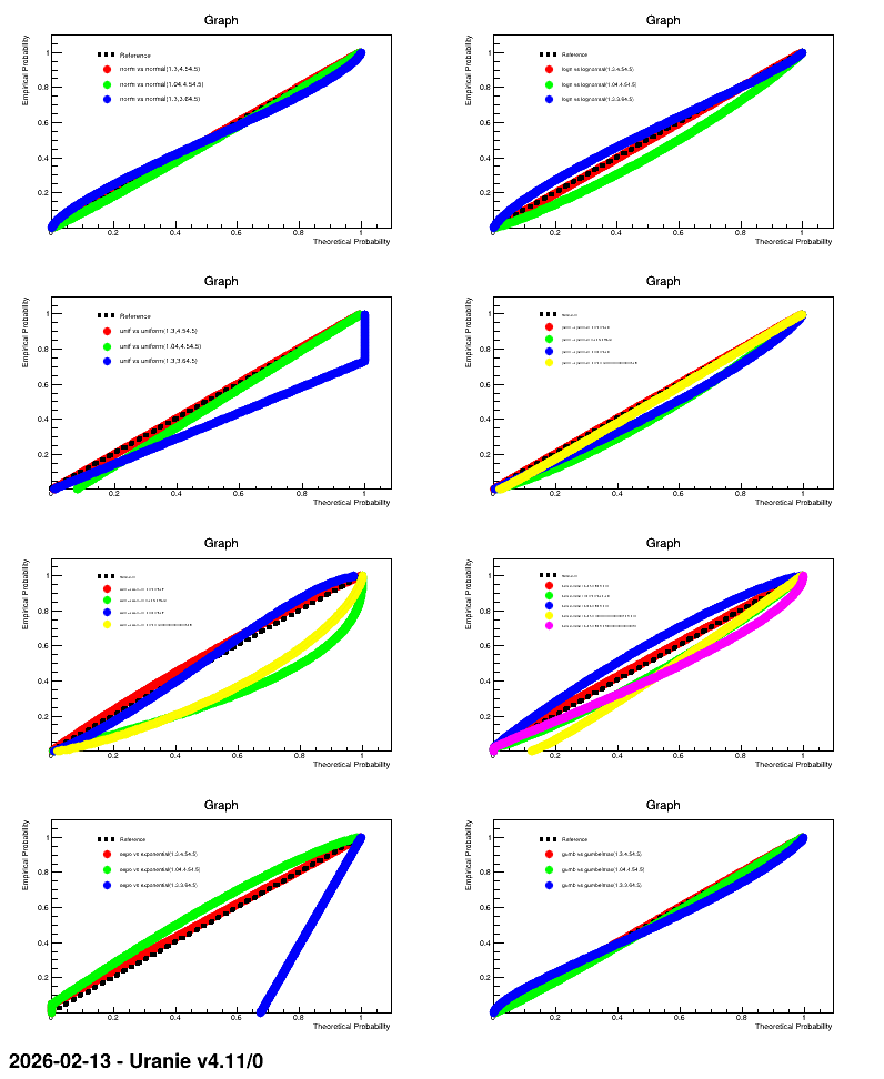"dataserverDrawPPPlot.py"