13.9.4. Macro “reoptimizeHollowBarVizirMoead.py”
13.9.4.1. Objective
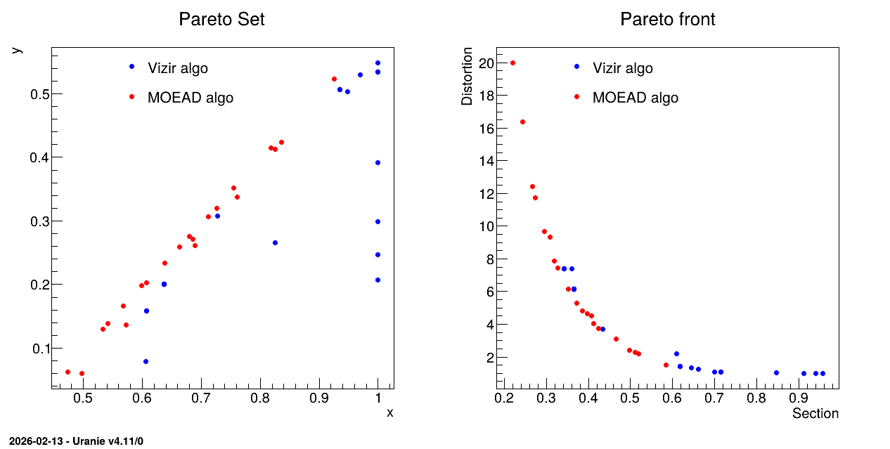
The objective of the macro is to optimize the section and distortion of the hollow bar defined in Sizing of a hollow bar example problem using the evolutionary solvers, with a reduce number of points to compose the Pareto set/front. This example is comparing both the usual Vizir genetic algorithm and the MOEAD implementation that is meant to be a many-objective criteria algorithm. A short discussion on the many-objective aspect can be found in [Bla17].
13.9.4.2. Macro Uranie
"""
Example of hollow bar optimisation with Moead approach
"""
from array import array
from URANIE import DataServer, Relauncher, Reoptimizer
import ROOT

# variables
x = DataServer.TAttribute("x", 0.0, 1.0)
y = DataServer.TAttribute("y", 0.0, 1.0)
thick = DataServer.TAttribute("thick")  # thickness
sect = DataServer.TAttribute("sect")  # section of the pipe
dist = DataServer.TAttribute("dist")  # distortion

ROOT.gROOT.LoadMacro("UserFunctions.C")

# Creating the assessor using the analytical function
code = Relauncher.TCIntEval("barAllCost")
code.addInput(x)
code.addInput(y)
code.addOutput(thick)
code.addOutput(sect)
code.addOutput(dist)

# Create a runner
runner = Relauncher.TSequentialRun(code)
runner.startSlave()  # Usual Relauncher construction

NB = 20
nMax = 3000
total = 4*NB
if runner.onMaster():
    # ==================================================
    # ========= Classical Vizir implementation =========
    # ==================================================

    # Create the TDS
    tds_viz = DataServer.TDataServer("vizirDemo", "Vizir parameter dataser")
    tds_viz.addAttribute(x)
    tds_viz.addAttribute(y)

    # create the vizir genetic solver
    solv_viz = Reoptimizer.TVizirGenetic()
    # Size of the population, and a maximum number of evaluation
    solv_viz.setSize(NB, nMax)

    # Create the multi-objective constrained optimizer
    opt_viz = Reoptimizer.TVizir2(tds_viz, runner, solv_viz)
    # add the objective
    opt_viz.addObjective(sect)  # minimizing the section
    opt_viz.addObjective(dist)  # minimizing the distortion

    # and the constrains
    positiv = Reoptimizer.TGreaterFit(0.4)
    opt_viz.addConstraint(thick, positiv)  # on thickness (thick > 0.4)

    opt_viz.solverLoop()  # running the optimization

    # ==================================================
    # ============== MOEAD implementation ==============
    # ==================================================

    # Create the TDS
    tds_moead = DataServer.TDataServer("vizirDemo", "Vizir parameter dataser")
    tds_moead.addAttribute(x)
    tds_moead.addAttribute(y)

    # create the vizir genetic solver
    solv_moead = Reoptimizer.TVizirGenetic()
    solv_moead.setMoeadDiversity(NB)
    solv_moead.setStoppingCriteria(1)
    solv_moead.setSize(0, nMax)

    # Create the multi-objective constrained optimizer
    opt_moead = Reoptimizer.TVizir2(tds_moead, runner, solv_moead)

    # add the objective
    opt_moead.addObjective(sect)  # minimizing the section
    opt_moead.addObjective(dist)  # minimizing the distortion

    opt_moead.addConstraint(thick, positiv)   # on thickness (thick > 0.4)

    opt_moead.solverLoop()  # running the optimization

    # Stop the slave processes
    runner.stopSlave()

    # Start the graphical part
    # Preparing canvas
    fig1 = ROOT.TCanvas("fig1", "Pareto Zone", 5, 64, 1270, 667)
    pad1 = ROOT.TPad("pad1", "", 0, 0.03, 1, 1)
    pad1.Draw()
    pad1.Divide(2, 1)
    pad1.cd(1)

    # extracting data to construct graphs
    viz = array('d', [0. for i in range(total)])
    # There is always one more point in moead
    moe = array('d', [0. for i in range(total+4)])
    tds_viz.getTuple().extractData(viz, total, "x:y:sect:dist", "", "column")
    tds_moead.getTuple().extractData(moe, total+4,
                                     "x:y:sect:dist", "", "column")

    set_viz = ROOT.TGraph(NB, array('d', [viz[i] for i in range(NB)]),
                          array('d', [viz[NB+i] for i in range(NB)]))
    fr_viz = ROOT.TGraph(NB, array('d', [viz[2*NB+i] for i in range(NB)]),
                         array('d', [viz[3*NB+i] for i in range(NB)]))
    set_viz.SetMarkerColor(4)
    set_viz.SetMarkerStyle(20)
    set_viz.SetMarkerSize(0.8)
    fr_viz.SetMarkerColor(4)
    fr_viz.SetMarkerStyle(20)
    fr_viz.SetMarkerSize(0.8)

    set_moe = ROOT.TGraph(NB+1, array('d', [moe[i] for i in range(NB+1)]),
                          array('d', [moe[NB+1+i] for i in range(NB+1)]))
    fr_moe = ROOT.TGraph(NB, array('d', [moe[2*(NB+1)+i] for i in range(NB+1)]),
                         array('d', [moe[3*(NB+1)+i] for i in range(NB+1)]))
    set_moe.SetMarkerColor(2)
    set_moe.SetMarkerStyle(20)
    set_moe.SetMarkerSize(0.8)
    fr_moe.SetMarkerColor(2)
    fr_moe.SetMarkerStyle(20)
    fr_moe.SetMarkerSize(0.8)

    # Legend
    ROOT.gStyle.SetLegendBorderSize(0)
    leg = ROOT.TLegend(0.25, 0.75, 0.55, 0.89)
    leg.AddEntry(set_viz, "Vizir algo", "p")
    leg.AddEntry(set_moe, "MOEAD algo", "p")

    # Pareto Set
    set_mg = ROOT.TMultiGraph()
    set_mg.Add(set_viz)
    set_mg.Add(set_moe)
    set_mg.Draw("aP")
    set_mg.SetTitle("Pareto Set")
    set_mg.GetXaxis().SetTitle("x")
    set_mg.GetYaxis().SetTitle("y")
    leg.Draw()
    ROOT.gPad.Update()

    # Pareto Front
    pad1.cd(2)
    fr_mg = ROOT.TMultiGraph()
    fr_mg.Add(fr_viz)
    fr_mg.Add(fr_moe)
    fr_mg.Draw("aP")
    fr_mg.SetTitle("Pareto front")
    fr_mg.GetXaxis().SetTitle("Section")
    fr_mg.GetYaxis().SetTitle("Distortion")
    leg.Draw()
    ROOT.gPad.Update()
The variables are defined as follow:
x = DataServer.TAttribute("x", 0.0, 1.0)
y = DataServer.TAttribute("y", 0.0, 1.0)
thick = DataServer.TAttribute("thick")  # thickness
sect = DataServer.TAttribute("sect")  # section of the pipe
dist = DataServer.TAttribute("dist")  # distortion
where the first two are the input ones while the last ones are computed using the provided code (as explained in Sizing of a hollow bar example problem). This code is configured through these lines
# Creating the assessor using the analytical function
code = Relauncher.TCIntEval("barAllCost")
code.addInput(x)
code.addInput(y)
code.addOutput(thick)
code.addOutput(sect)
code.addOutput(dist)
The usual Relauncher construction is followed, using a TSequentialRun runner. The first solver is
defined in these lines
# create the vizir genetic solver
solv_viz = Reoptimizer.TVizirGenetic()
# Size of the population, and a maximum number of evaluation
solv_viz.setSize(NB, nMax)
Combining the runner, solver and dataserver, the master object is created and the objective and constraint are defined. This is done in:
# Create the multi-objective constrained optimizer
opt_viz = Reoptimizer.TVizir2(tds_viz, runner, solv_viz)
# add the objective
opt_viz.addObjective(sect)  # minimizing the section
opt_viz.addObjective(dist)  # minimizing the distortion

# and the constrains
positiv = Reoptimizer.TGreaterFit(0.4)
opt_viz.addConstraint(thick, positiv)  # on thickness (thick > 0.4)
In a second block a new dataserver is created along with a new genetic solver in these lines:
# create the vizir genetic solver
solv_moead = Reoptimizer.TVizirGenetic()
solv_moead.setMoeadDiversity(NB)
solv_moead.setStoppingCriteria(1)
solv_moead.setSize(0, nMax)
The idea here is to use the Moead algorithm whose principle in few words is to split the space into
a certain numbers of direction intervals (set by the argument in the function setMoeadDiversity).
This should provide a Pareto front with a better homogeneity in the front member distribution
(particularly visible here when the size of the requested ensemble is small). The second method,
setStoppingCriteria(1) states that the only stopping criteria available is the total number of
estimation, allowed in the setSize method. Finally, the last function to be called is the setSize
one, with a peculiar first argument here: the size of the pareto can be chosen but if 0 is put (as
done here) the number of elements will be the number of intervals defined previously plus one (the
plus one comes from the fact that the elements are created at the edge of every interval, so for 20
intervals, there are 21 edges in total).
The rest of the code is creating the plot shown below in which both Pareto set and front are compared.
13.9.4.3. Graph
Figure 13.56 Graph of the macro “reoptimizeHollowBarVizirMoead.py”