3.2.4.1. Introduction

Considering the definition of a LHS sampling, introduced in Introduction and also discussed in Introduction, it is clear that permutating a coordinate of two different points, will create a new sampling. The idea here is to use this already discussed property to create fulfill requested constraints on the design-of-experiments to be produced. Practically, the constraint will have one main limitation: it should only imply two variables. This limitation is set, so far, for simplicity purpose, as the constraint matrix might blow up and the solutions in term of permutation will also become very complicated (see the heuristic description below in The heuristic to get a glimpse at the possible complexity).

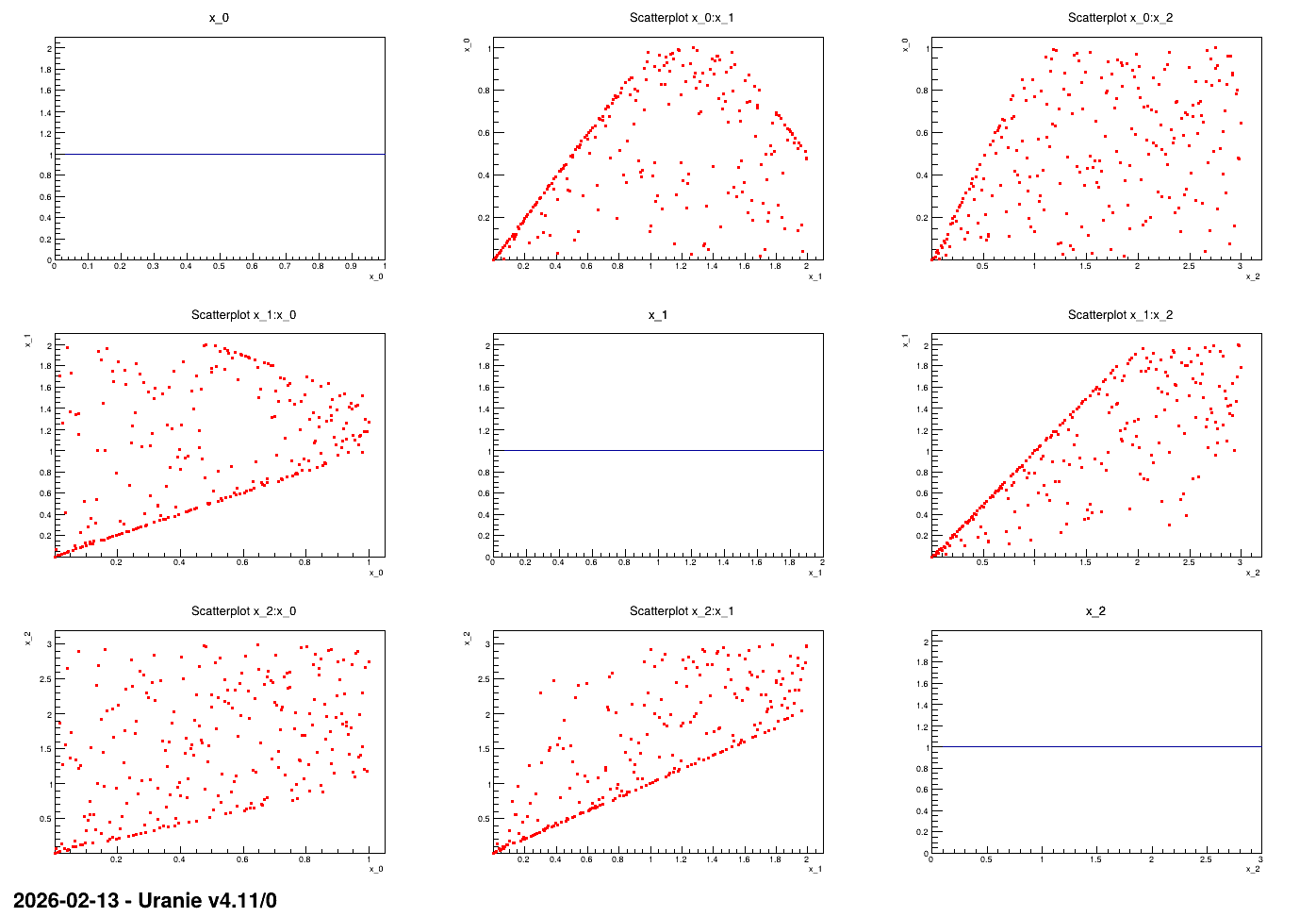
Before this algorithm, the solution to be sure to fulfill a constraint was to generate a large sample and apply the constraint as a cut, meaning that no control on the final number of locations in the design-of-experiments and on the marginal distribution shape was possible. From a theoretical perspective, using a constrained LHS is allowing both to have the correct expected marginal distributions and to have precisely the requested number of locations to be submitted to a code or function. This is shown in Figure 3.5, where in a simple case with only three variables uniformly distributed, it is possible to apply three linear constraints: two of them are applied on the \((x_0, x_1)\) plane while the last one is applied on the \((x_1, x_2)\) one.

Figure 3.5 Matrix of distribution of three uniformly distributed variables on which three linear constraints are applied. The diagonal are the marginal distributions while the off-diagonal are the two-by-two scatter plots.