2.1.1.6. LogNormal law

If a random variable \(x\) follows a LogNormal distribution, the random variable \(\ln(x)\) follows a Normal distribution (whose parameters are \(\mu\) and \(\sigma\)), so

\[f(x) = \frac{1}{(x-x_{\rm min})\sigma\sqrt{2\pi}} \times e^{\frac{-(\ln(x-x_{\rm min})-\mu)^{2}} {2\sigma^{2}}} \; {\rm1\kern-0.28emI}_{[x_{\rm min},+\infty[}(x)\]

In Uranie, it is parametrised by default using \(M\), the mean of the distribution, \(E_{f}\), the Error factor that represents the ration of the 95% quantile and the median (\(E_{f} = q_{0.95} / q_{0.50}\)) and the minimum \(x_{\rm min}\). One can go from one parametrisation to the other following those simple relations

\[\begin{split}\begin{array}{ccc} M = e^{\mu + \sigma^2/2} + x_{\rm min} & \Leftrightarrow & \mu = \ln{(M-x_{\rm min})} - \sigma^{2}/2 \\ E_{F} = e^{1.645\times\sigma} & \Leftrightarrow & \sigma = \ln{(E_{f})}/1.645\\ \end{array}\end{split}\]

The variance of the distribution can be estimated as \({\rm Var}=(e^{\sigma^2}-1)e^{2\mu+\sigma^2} = (e^{(\frac{\ln{(E_{f})}}{1.645})^2}-1)\times (M-x_{\rm min})^{2}\) while its mean is \(e^{\mu + \sigma^2/2}\) and its mode is \(e^{\mu - \sigma^2}\).

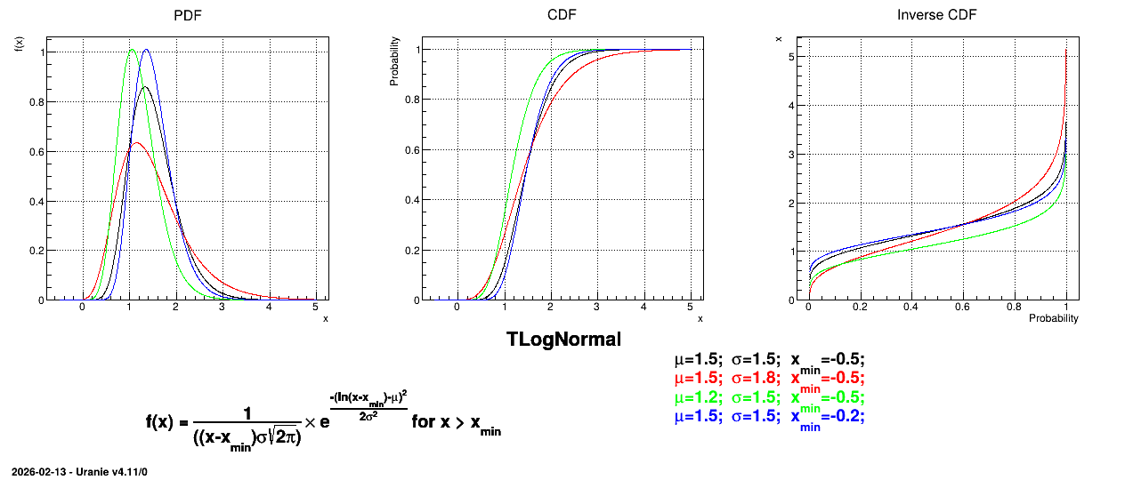
Figure 2.7 shows the PDF, CDF and inverse CDF generated for different sets of parameters.

Figure 2.7 Example of PDF, CDF and inverse CDF for LogNormal distributions.