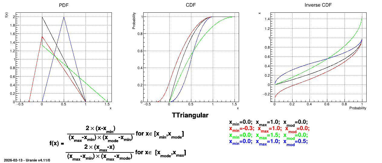
2.1.1.3. Triangular Law

This law describes a triangle with a base between a minimum and a maximum and a highest density at a certain point \(x_{\rm mode}\), so

\[f(x) = \frac{2 \times (x-x_{\rm min})}{ (x_{\rm max}-x_{\rm min}) \times (x_{\rm mode}-x_{\rm min}) } {\rm 1\kern-0.28emI}_{[x_{\rm min}, x_{\rm mode}]}(x)\]

and

\[f(x) = \frac{2 \times (x_{\rm max}-x)}{ (x_{\rm max}-x_{\rm min}) \times (x_{\rm max}-x_{\rm mode}) } {\rm 1\kern-0.28emI}_{[x_{\rm mode},x_{\rm max}]}(x)\]

The mean value of the triangular law can then be computed as \(\mu = \dfrac{x_{\rm max}+x_{\rm min}+ x_{\rm mode}}{3}\) while its variance can be written as \(\sigma^2=\dfrac{(x^{2}_{\rm max}+ x^{2}_{\rm min}+x^{2}_{\rm mode}-x_{\rm max}x_{\rm min}-x_{\rm max}x_{\rm mode}-x_{\rm mode} x_{\rm min})}{18} \).

Figure 2.4 shows the PDF, CDF and inverse CDF generated for different sets of parameters.

Figure 2.4 Example of PDF, CDF and inverse CDF for Triangular distributions.