2.2.5.18. Generalized normal law

This law describes a generalized normal distribution depending on the location \(\mu\), the scale \(\alpha\) and the shape \(\beta\), as

\[f(x) = \frac{\beta}{2 \alpha \Gamma \left(1/\beta \right) } \times e^{-\left(\frac{x-\mu}{\alpha} \right)^{\beta}}\]

Both \(\alpha\) and \(\beta\) should be greater than 0.

Uranie code to simulate a generalized normal random variable is:

    TDataServer *tds = new TDataServer("tdssampler", "Sampler Uranie demo");
    tds->addAttribute( new TGeneralizedNormalDistribution("gennor", 0.0, 1.0, 3.0) );
    
    TSampling *fsamp = new TSampling(tds, "lhs", 300);
    fsamp->generateSample(); // Create a representative sample
    
    tds->Draw("gennor");

Figure 2.32 shows the PDF, CDF and inverse CDF generated for different sets of parameters.

../../../_images/TGeneralizedNormalDistribution.png — Figure 2.32 Example of PDF, CDF and inverse CDF for GeneralizedNormal distributions.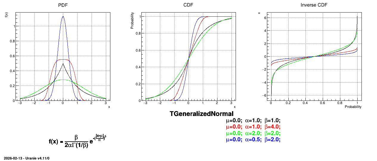

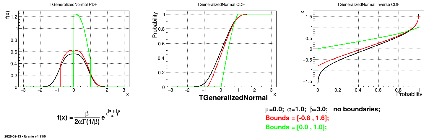
Is it also possible to set boundaries to the infinite span of this distribution to create a truncated generalized normal law. This can be done by calling the following method:

    tds->getAttribute("gennor")->setBounds(-0.8,1.6); //truncate the law

The resulting PDF, CDF and inverse CDF, with and without truncation, can be seen, in this case, in Figure 2.33 for a given set of parameters and various boundaries.