2.2.5.3. Triangular Law

This law describes a triangle with a base between a minimum and a maximum and a highest density at a certain point \(x_{\rm mode}\), so

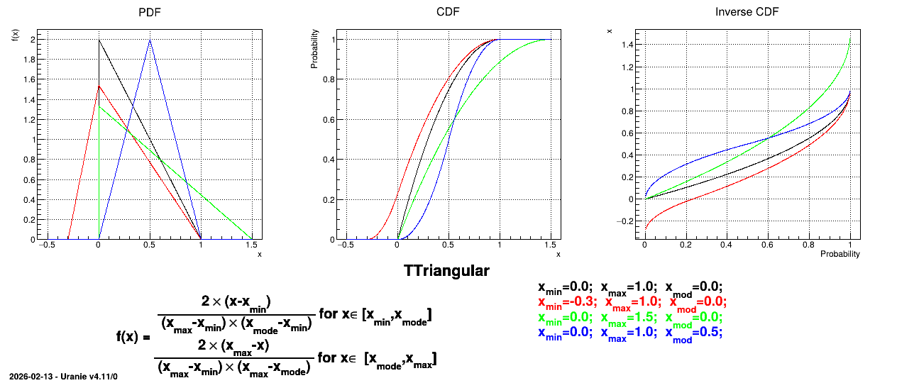
\[f(x) = \frac{2 \times (x-x_{\rm min})}{ (x_{\rm max}-x_{\rm min}) \times (x_{\rm mode}-x_{\rm min}) } {\rm 1\kern-0.28emI}_{[x_{\rm min}, x_{\rm mode}]}(x)\]

and

\[f(x) = \frac{2 \times (x_{\rm max}-x)}{ (x_{\rm max}-x_{\rm min}) \times (x_{\rm max}-x_{\rm mode}) } {\rm 1\kern-0.28emI}_{[x_{\rm mode},x_{\rm max}]}(x)\]

Uranie code to simulate a triangular random variable is:

    TDataServer *tds = new TDataServer("tdssampler", "Sampler Uranie demo");
    tds->addAttribute( new TTriangularDistribution("t", 5.0, 8., 6.0));
    
    TSampling *fsamp = new TSampling(tds, "lhs", 300);
    fsamp->generateSample(); // Create a representative sample
    
    tds->Draw("t");

Figure 2.7 shows the PDF, CDF and inverse CDF generated for different sets of parameters.