13.10.1. Macro “calibrationMinimisationFlowrate1D.C”

13.10.1.1. Objective

The goal here is to calibrate the parameter \(H_l\) within the flowrate model, while varying only two inputs (\(r_{\omega}\) and \(L\)). The remaining variables are fixed to the following values: \(r=25050\), \(T_u=89335\), \(T_l=89.55\), \(H_u=1050\), \(K_{\omega}=10950\). The context of this example has already been presented in Use-case for this chapter, including the model (implemented here as a C++ function) and the initial lines defining the TDataServer objects. This macro demonstrates how to apply a simple minimisation approach using a Relauncher-based architecture.

13.10.1.2. Macro Uranie

    TDataServer *tdsRef = new TDataServer("tdsRef","doe_exp_Re_Pr");
    TDataServer *tdsPar = new TDataServer("tdsPar","tdsPar");

    TCanvas *canRes = new TCanvas("CanRes","CanRes",1200,800);
    TPad *apad = new TPad("apad","apad",0, 0.03, 1, 1);

    // Load the function flowrateCalib1D
    gROOT->LoadMacro("UserFunctions.C");
    
    // Input reference file   
    TString ExpData="Ex2DoE_n100_sd1.75.dat";

    // define the reference
    tdsRef->fileDataRead(ExpData.Data());
    
    // define the parameters
    tdsPar->addAttribute( new TAttribute("hl", 700.0, 760.0) );
    tdsPar->getAttribute("hl")->setDefaultValue(728.0);
    
    // Create the output attribute
    TAttribute *out = new TAttribute("out");
    
    // Create interface to assessors
    TCIntEval *Model = new TCIntEval("flowrateCalib1D");
    Model->addInput(tdsPar->getAttribute("hl"));
    Model->addInput(tdsRef->getAttribute("rw"));
    Model->addInput(tdsRef->getAttribute("l"));
    Model->addOutput(out);
    
    // Set the runner
    TSequentialRun *runner = new TSequentialRun(Model);    
    
    // Set the calibration object
    TMinimisation *cal = new TMinimisation(tdsPar,runner,1);
    cal->setDistance("LS",tdsRef,"rw:l","Qexp");
    TNloptSubplexe solv;
    cal->setOptimProperties(&solv);
    cal->estimateParameters();
    
    // Draw the residuals
    apad->Draw();
    apad->cd();
    cal->drawResiduals("Residuals","*","","nonewcanvas");

Apart from the initial lines described in the section Use-case for this chapter, the key step is to define the starting point of the minimisation. This can be achieved either by calling the setStartingPoint method of the TNlopt class, or by assigning a default value to the parameter attributes. In this example, it is done as follows:

    tdsPar->getAttribute("hl")->setDefaultValue(728.0);

The model is defined (from a TCIntEval instance with the three input variables discussed above, in the correct order) along with the computation distribution method (sequential).

    // Create interface to assessors
    TCIntEval *Model = new TCIntEval("flowrateCalib1D");
    Model->addInput(tdsPar->getAttribute("hl"));
    Model->addInput(tdsRef->getAttribute("rw"));
    Model->addInput(tdsRef->getAttribute("l"));
    Model->addOutput(out);
    
    // Set the runner
    TSequentialRun *runner = new TSequentialRun(Model);    

Once this setup is complete, the calibration object (TMinimisation) is created. As explained in Recommended distance and likelihood functions, construction method, the first step is to define the distance function (here the least squares distance) using setDistance. This method also specifies the TDataServer containing the reference data, the names of the reference inputs, and the reference variable against which the model output is compared. Finally, the optimisation algorithm is defined by creating an instance of TNloptSubplexe, and the parameters are then estimated.

    // Set the calibration object
    TMinimisation *cal = new TMinimisation(tdsPar,runner,1);
    cal->setDistance("LS",tdsRef,"rw:l","Qexp");
    TNloptSubplexe solv;
    cal->setOptimProperties(&solv);
    cal->estimateParameters();

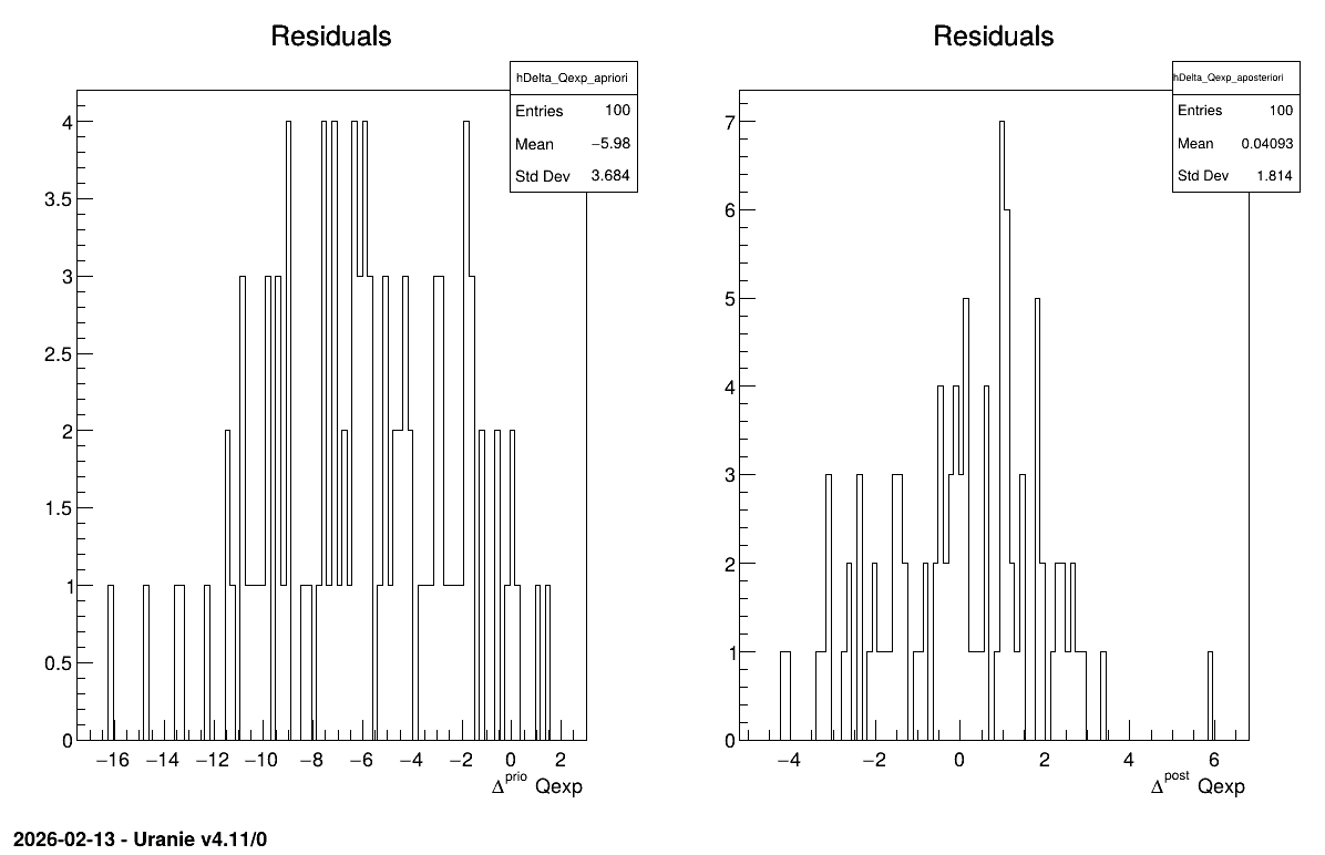
The final part demonstrates how to display the results. Since this method produces a point estimate, only a single value is obtained, which is always shown on the screen, as illustrated in Console. Another important aspect is to examine the residuals, as discussed in [Bla17]. This is illustrated in Figure 13.60, which shows the residuals of the a posteriori estimates, typically following a normal distribution.

    // Draw the residuals
    apad->Draw();
    apad->cd();
    cal->drawResiduals("Residuals","*","","nonewcanvas");

13.10.1.3. Console

--- Uranie v4.11/0 --- Developed with ROOT (6.36.06)
                      Copyright (C) 2013-2026 CEA/DES 
                      Contact: support-uranie@cea.fr 
                      Date: Thu Feb 12, 2026

|....:....|....:....|....:....|....:
.************************************************
*    Row   * tdsPar__n *     hl.hl * agreement *
************************************************
*        0 *         0 * 749.72363 * 18.149368 *
************************************************

13.10.1.4. Graph

Figure 13.60 Residuals graph of the macro “calibrationMinimisationFlowrate1D.C”