13.2.8. Macro “dataserverComputeQuantile.C”

13.2.8.1. Objective

The objective of this macro is to test the classical quantile estimation and compare it to the Wilks estimation for a dummy gaussian distribution. Four different estimations of the 95% quantile value are done (along with one estimation of th 99% quantile) for illustration purposes:

• using the usual method with a 200-points sample.

• using the usual method with a 400-points sample.

• using the Wilks method with a 95% confidence level (with 59-points sample).

• using the Wilks method with a 95% confidence level (with 400-points sample).

• using the Wilks method with a 99% confidence level (with 90-points sample).

13.2.8.2. Macro Uranie

    //Create a DataServer
    TDataServer *tds = new TDataServer("foo","pouet");

    gStyle->SetOptStat(0);
    TCanvas *can = new TCanvas("Can","Can",10,10,1000,1000);

    tds->addAttribute("x"); //With one attribute

    //Create Histogram to store the quantile values
    TH1F *Q200 = new TH1F("quantile200","",60,1,4); Q200->SetLineColor(1); Q200->SetLineWidth(2);
    TH1F *Q400 = new TH1F("quantile400","",60,1,4); Q400->SetLineColor(4); Q400->SetLineWidth(2);
    TH1F *QW95 = new TH1F("quantileWilks95","",60,1,4); QW95->SetLineColor(2); QW95->SetLineWidth(2);
    TH1F *QW95400 = new TH1F("quantileWilks95400","",60,1,4); QW95400->SetLineColor(8); QW95400->SetLineWidth(2);
    TH1F *QW99 = new TH1F("quantileWilks99","",60,1,4); QW99->SetLineColor(6); QW99->SetLineWidth(2);

    //Defining the sample size
    int nb[4] = {200,400,59,90};
    double quant=0.95; //Quantile value
    double CL[2] = {0.95, 0.99};//Confidence level value for the two Wilks computation
    //Loop over the number of estimation (2 usual with different number of sample and 1 with Wilks estimation)
    for(unsigned int iq=0; iq<4; iq++)
    {
        //Produce 10000 drawing to get smooth distributio,
        for(unsigned int itest=0; itest < 10000; itest++)
        {
            tds->createTuple(); // Create the tuple to store value

            // Fill it with random drawing of centered gaussian
            for(unsigned int ival=0; ival < nb[iq]; ival++)
                tds->getTuple()->Fill(ival+1, gRandom->Gaus(0,1) );

            // Estimate the quantile...
            double value;
            if (iq<2)
            {
                // ... with usual methods...
                tds->computeQuantile("x",quant, value);
                if(iq==0) Q200->Fill(value); // ... on a 200-points sample
                else
                {
                    Q400->Fill(value); // ... on a 400-points sample
             tds->estimateQuantile("x", quant, value, CL[iq-1]);
             QW95400->Fill(value); // compute the quantile at 95% CL
                }
            }
            else
            {
                // ... with the wilks optimised sample
                tds->estimateQuantile("x", quant, value, CL[iq-2]);
                if(iq==2) QW95->Fill(value); // compute the quantile at 95% CL
                else QW99->Fill(value); // compute the quantile at 99% CL
            }

            // Delete the tuple
            tds->deleteTuple();
        }
    }

    //Produce the plot with requested style
    Q400->GetXaxis()->SetTitle("Quant_{95%}(Gaus_{(0,1)})");
    Q400->GetXaxis()->SetTitleOffset(1.2);
    Q400->Draw();
    Q200->Draw("same");
    QW95->Draw("same");
    QW95400->Draw("same");
    QW99->Draw("same");

    //Add the theoretical estimation
    TLine *lin = new TLine(); lin->SetLineStyle(3);
    lin->DrawLine(1.645,0,1.645, Q400->GetMaximum());

    //Add a block of legend
    TLegend *leg = new TLegend(0.4,0.6,0.8,0.85);
    leg->AddEntry(lin,"Theoretical quantile","l");
    leg->AddEntry(Q200, "Usual quantile (200 pts)","l");
    leg->AddEntry(Q400, "Usual quantile (400 pts)","l");
    leg->AddEntry(QW95, "Wilks quantile CL=95% (59 pts)","l");
    leg->AddEntry(QW95400, "Wilks quantile CL=95% (400 pts)","l");
    leg->AddEntry(QW99, "Wilks quantile CL=99% (90 pts)","l");
    leg->SetBorderSize(0);
    leg->Draw();

In this macro, a dummy dataserver is created with a single attribute named “x”. Four histograms are prepared to store the resulting value. Then the same loop will be used to computed 10000 values of every quantile with different switchs to use one method instead of the other, or to change the number of points in the sample and/or the confidence level. All this is defined in the small part before the loop:

    //Defining the sample size
    int nb[4] = {200,400,59,90};
    double quant=0.95; //Quantile value
    double CL[2] = {0.95, 0.99};//Confidence level value for the two Wilks computation

Then the computation is performed, first for the usual method (first two iterations of iq), then for the Wilks estimation (last two iterations of iq). Every computational result is stored in the corresponding histogram which is finally displayed and shown in the following subsection.

13.2.8.3. Graph

Figure 13.6 Graph of the macro 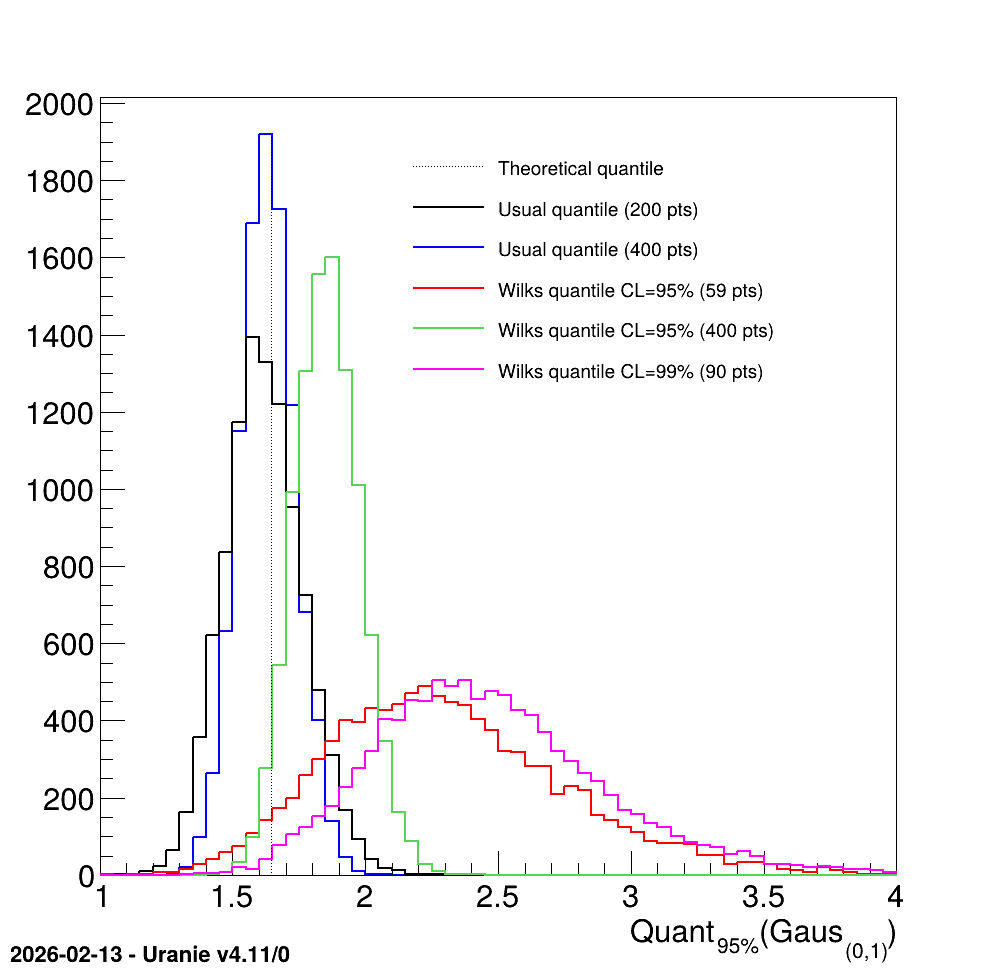"dataserverComputeQuantile.C"