13.2.15. Macro “dataserverDrawQQPlot.C”

13.2.15.1. Objective

This macro is an example of how to produce QQ-plot for a certain number of randomly-drawn samples, providing the correct parameter values along with modified versions to illustrate the impact.

13.2.15.2. Macro Uranie

    TDataServer *tds0 = new TDataServer();

    //Create the canvas
    TCanvas *c = new TCanvas("c1","",800,1000);
    TPad *apad = new TPad("apad","apad",0, 0.03, 1, 1);

    // Create a TDS with 8 kind of distributions
    double p1=1.3, p2=4.5, p3=0.9, p4=4.4; // Fixed values for parameters
    
    tds0->addAttribute(new TNormalDistribution("norm", p1, p2));
    tds0->addAttribute(new TLogNormalDistribution("logn", p1, p2));
    tds0->addAttribute(new TUniformDistribution("unif", p1, p2));
    tds0->addAttribute(new TExponentialDistribution("expo", p1, p2));
    tds0->addAttribute(new TGammaDistribution("gamm", p1, p2, p3));
    tds0->addAttribute(new TBetaDistribution("beta", p1, p2, p3, p4));
    tds0->addAttribute(new TWeibullDistribution("weib", p1, p2, p3));
    tds0->addAttribute(new TGumbelMaxDistribution("gumb", p1, p2));
     
    // Create the sample
    TBasicSampling *fsamp = new TBasicSampling(tds0, "lhs", 200);
    fsamp->generateSample();

    // Define number of laws, their name and numbers of parameters
    unsigned int nLaws=8;
    string laws[8]={"normal", "lognormal", "uniform", "gamma", "weibull", "beta", "exponential", "gumbelmax"}; // number of parameters to put in () for the corresponding law
    int npar[8]={2, 2, 2, 3, 3, 4, 2, 2};
    
    //Create the 8 pads
    apad->Draw();
    apad->cd();
    apad->Divide(2,4);

    // Number of points to compare theoretical and empirical values
    int nS=1000;
    double mod=0.8; // Factor used to artificially change the parameter values
    
    TString opt=""; //option of the drawQQPlot method
    stringstream sstr;
    for(unsigned int ilaw=0; ilaw<nLaws; ilaw++)
    {
        // Clean sstr
        sstr.str("");
        // Add nominal configuration
        sstr << laws[ilaw] << "("<<p1<<","<<p2<<((npar[ilaw]>=3)?Form(",%g",p3):"")<<p2<<((npar[ilaw]>=4)?Form(",%g",p4):"")<<")";
        // Changing par1
        sstr << ":" << laws[ilaw] << "("<<p1*mod<<","<<p2<<((npar[ilaw]>=3)?Form(",%g",p3):"")<<p2<<((npar[ilaw]>=4)?Form(",%g",p4):"")<<")";
        // Changing par2
        sstr << ":" << laws[ilaw] << "("<<p1<<","<<p2*mod<<((npar[ilaw]>=3)?Form(",%g",p3):"")<<p2<<((npar[ilaw]>=4)?Form(",%g",p4):"")<<")";
        // Changing par3
        if(npar[ilaw] >=3 )
            sstr << ":" << laws[ilaw] << "("<<p1<<","<<p2<<((npar[ilaw]>=3)?Form(",%g",p3*mod):"")<<p2<<((npar[ilaw]>=4)?Form(",%g",p4):"")<<")";
        // Changing par4
        if(npar[ilaw] >=4 )
            sstr << ":" << laws[ilaw] << "("<<p1<<","<<p2<<((npar[ilaw]>=3)?Form(",%g",p3):"")<<p2<<((npar[ilaw]>=4)?Form(",%g",p4*mod):"")<<")";
        //cout<<sstr.str()<<endl;

        apad->cd(ilaw+1);
        // Produce the plot
        tds0->drawQQPlot( laws[ilaw].substr(0,4).c_str(), sstr.str().c_str(), nS, opt);
    }

The very first step of this macro is to create a sample that will contain a design-of-experiments filled with 200 locations, using various statistical laws. All the tested laws, are those available in the drawQQPlot method and they might depend on 2 to 4 parameters, defined a but randomly at the beginning of this piece of code.

    TDataServer *tds0 = new TDataServer();

    // Create a TDS with 8 kind of distributions
    double p1=1.3, p2=4.5, p3=0.9, p4=4.4; // Fixed values for parameters
    
    tds0->addAttribute(new TNormalDistribution("norm", p1, p2));
    tds0->addAttribute(new TLogNormalDistribution("logn", p1, p2));
    tds0->addAttribute(new TUniformDistribution("unif", p1, p2));
    tds0->addAttribute(new TExponentialDistribution("expo", p1, p2));
    tds0->addAttribute(new TGammaDistribution("gamm", p1, p2, p3));
    tds0->addAttribute(new TBetaDistribution("beta", p1, p2, p3, p4));
    tds0->addAttribute(new TWeibullDistribution("weib", p1, p2, p3));
    tds0->addAttribute(new TGumbelMaxDistribution("gumb", p1, p2));

Once done, the sample is generated using TBasicSampling object with an LHS algorithm. On top of this, despite the plot preparation with canvas and pad generation, several variables are set to prepare the tests, as shown below

    // Define number of laws, their name and numbers of parameters
    unsigned int nLaws=8;
    string laws[8]={"normal", "lognormal", "uniform", "gamma", "weibull", "beta", "exponential", "gumbelmax"}; // number of parameters to put in () for the corresponding law
    int npar[8]={2, 2, 2, 3, 3, 4, 2, 2};
    
    // Number of points to compare theoretical and empirical values
    int nS=1000;
    double mod=0.8; // Factor used to artificially change the parameter values

Finally, after the line of hypothesis to be tested is constructed (the first paragraph in the for loop) the drawQQPlot method is called for every empirical law in the following line.

        tds0->drawQQPlot( laws[ilaw].substr(0,4).c_str(), sstr.str().c_str(), nS, opt);

For the first case, when one wants to test the TNormalDistribution “norm” with the known parameters and a variation of each, it resumes as if this line was run:

    tds0->drawQQPlot( "norm", "normal(1.3,4.5):normal(1.04,4.5):normal(1.3,3.6)", nS);

The first field is the attribute to be tested, while the second one provides the three hypothesis with which our attribute under investigation will be compared. The third argument is the number of steps to be computed for quantiles.

The result of this macro is shown below.

13.2.15.3. Graph

Figure 13.7 Graph of the macro 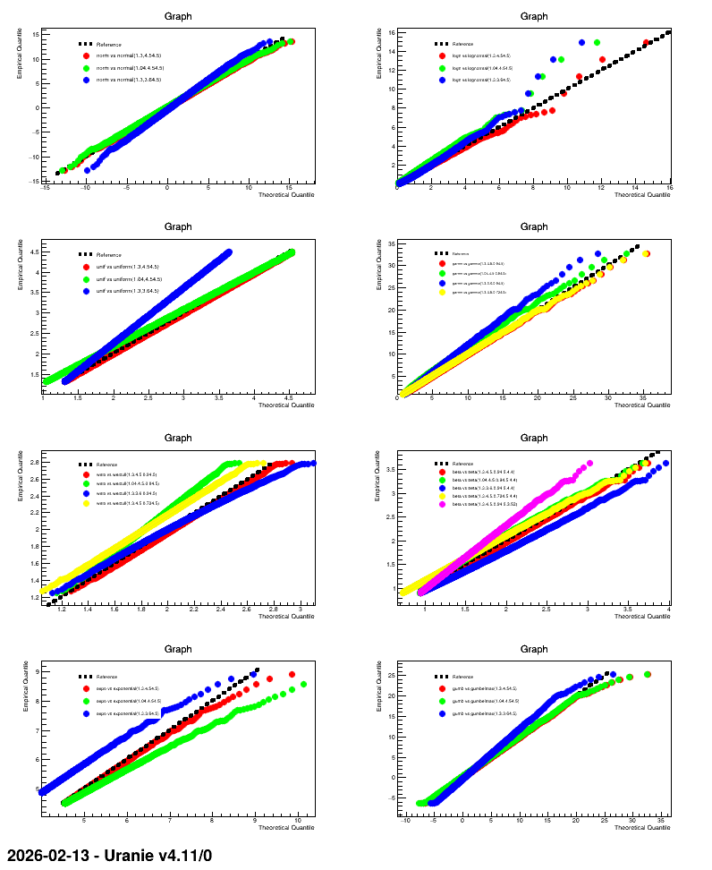"dataserverDrawQQPlot.C"