2.2.5.19. Composing law
It is possible to imagine a new law, hereafter called composed law, by combining different pre-existing laws in order to model a wanted behaviour. This law would be defined with \(N\) pre-existing laws whose densities are noted \(\lbrace f_j\rbrace_{1\leq j \leq N }\), along with their relative weights \(\lbrace \omega_j\rbrace_{1\leq j \leq N } \in (\mathbb{R}^{+})^{N}\) and the resulting density is then written as
Uranie code to simulate a composition of three normally-distributed laws (with their own statistical properties):
tds = DataServer.TDataServer("tdssampler", "Sampler Uranie demo")
comp = DataServer.TComposedDistribution("compo")
comp.addDistribution(DataServer.TNormalDistribution("n1", -1.5, 0.2), 1.2)
comp.addDistribution(DataServer.TNormalDistribution("n2", 0, 0.5), 1.0)
comp.addDistribution(DataServer.TNormalDistribution("n3", 1.5, 0.2), 0.8)
tds.addAttribute(comp)

fsamp = Sampler.TSampling(tds, "lhs", 300)
fsamp.generateSample()  # Create a representative sample

tds.Draw("compo")
Figure 2.34 shows the PDF, CDF and inverse CDF generated for different sets of parameters.
Figure 2.34 Example of PDF, CDF and inverse CDF for a composed distribution made out of three normal
distributions with respective weights.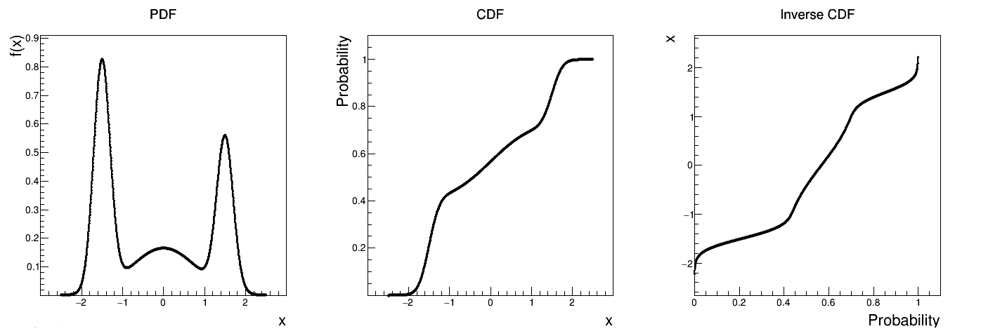
Is it also possible to set boundaries to the infinite span of this distribution, if it is created from at least one infinite-based law, to create a truncated composed law. This can be done by calling the following method:
tds.getAttribute("compo").setBounds(-1.6,1.8) # truncate the law
The resulting PDF, CDF and inverse CDF, with and without truncation, can be seen, in this case, in Figure 2.35 for a given set of parameters and various boundaries.
Figure 2.35 Example of PDF, CDF and inverse CDF for a truncated composed distribution made out of three
normal distributions with respective weights.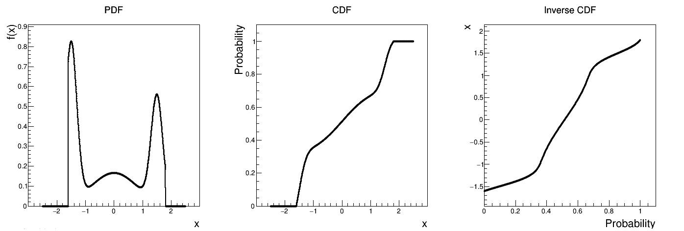
The only specific method that is new for the composition is the addDistribution method whose
signature is the following one:
addDistribution(statt, weight=1.)
The first element is a pointer to a TStochasticAttribute (so any object that is an instance of a
class that derives form it). The second one is the weight (which is 1 by default) and which is the
\(\omega\) constant written in the formula above.
Warning
The theoretical element (mean, standard deviation and mode) can not always be measured for certain stochastic distribution (see the Cauchy’s one for instance).
If one wants to add such a distribution in a composed law, a warning exception should pop-up to state that theoretical properties can not be estimated.
As for the mode, several distributions prevent from having a single-point mode estimation (for instance the Uniform distribution). The mode estimation should then be taken with great care.