2.2.5.6. LogNormal law

If a random variable \(x\) follows a LogNormal distribution, the random variable \(\ln(x)\) follows a Normal distribution (whose parameters are \(\mu\) and \(\sigma\)), so

\[f(x) = \frac{1}{(x-x_{\rm min})\sigma\sqrt{2\pi}} \times e^{\frac{-(\ln(x-x_{\rm min})-\mu)^{2}} {2\sigma^{2}}} \; {\rm1\kern-0.28emI}_{[x_{\rm min},+\infty[}(x)\]

In Uranie, it is parametrised by default using \(M\), the mean of the distribution, \(E_{f}\), the Error factor that represents the ration of the 95% quantile and the median (\(E_{f} = q_{0.95} / q_{0.50}\)) and the minimum \(x_{\rm min}\). One can go from one parametrisation to the other following those simple relations

\[\begin{split}\begin{array}{ccc} M = e^{\mu + \sigma^2/2} + x_{\rm min} & \Leftrightarrow & \mu = \ln{(M-x_{\rm min})} - \sigma^{2}/2 \\ E_{F} = e^{1.645\times\sigma} & \Leftrightarrow & \sigma = \ln{(E_{f})}/1.645\\ \end{array}\end{split}\]

Uranie code to simulate a LogNormal random variable is:

tds = DataServer.TDataServer("tdssampler", "Sampler Uranie demo")
# using M, Ef and xmin
tds.addAttribute(DataServer.TLogNormalDistribution("ln", 1.2, 1.5, -0.5))  
# to use ln(x) properties:
# mu = 0.5
# sigma = 1
# tds.setUnderlyingNormalParameters(mu,sigma)  

fsamp = Sampler.TSampling(tds, "lhs", 300)
fsamp.generateSample()  # Create a representative sample

tds.Draw("ln")
tds.Draw("log(ln)")  # Check that ln(ln) follows a normal law

Figure 2.11 shows the PDF, CDF and inverse CDF generated for different sets of parameters.

../../../_images/TLogNormalDistribution.png — Figure 2.11 Example of PDF, CDF and inverse CDF for LogNormal distributions.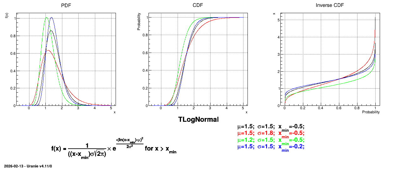

Is it also possible to set boundaries to the infinite span of this distribution to create a truncated normal law. This can be done by calling the following method:

tds.getAttribute("ln").setBounds(0.6,3.1)  # truncate the law

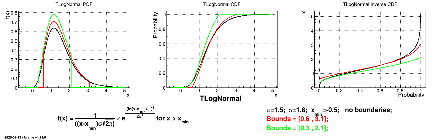
The resulting PDF, CDF and inverse CDF, with and without truncation, can be seen, in this case, in Figure 2.12 for a given set of parameters and various boundaries.