2.2.5.15. Gamma law

The Gamma distribution is a two-parameter family of continuous probability distributions. It depends on a shape parameter \(\alpha\) and a scale parameter \(\beta\). The function is usually defined for \(x\) greater than 0, but the distribution can be shifted thanks to the third parameter called location (\(\xi\)) which should be positive. This parametrisation is more common in Bayesian statistics, where the gamma distribution is used as a conjugate prior distribution for various types of laws:

\[f(x) = \frac{(x-\xi)^{\alpha - 1} e^{-(x-\xi)/\beta}}{ \Gamma(\alpha) \beta^{\alpha}} \; {\rm 1\kern-0.28emI}_{]\xi,+\infty]}(x)\]

Uranie code to simulate a Gamma random variable is:

tds = DataServer.TDataServer("tdssampler", "Sampler Uranie demo")
tds.addAttribute(DataServer.TGammaDistribution("gam", 1.0, 2.0, 0.0))

fsamp = Sampler.TSampling(tds, "lhs", 300)
fsamp.generateSample()  # Create a representative sample

tds.Draw("gam")

Figure 2.26 shows the PDF, CDF and inverse CDF generated for different sets of parameters.

../../../_images/TGammaDistribution.png — Figure 2.26 Example of PDF, CDF and inverse CDF for Gamma distributions.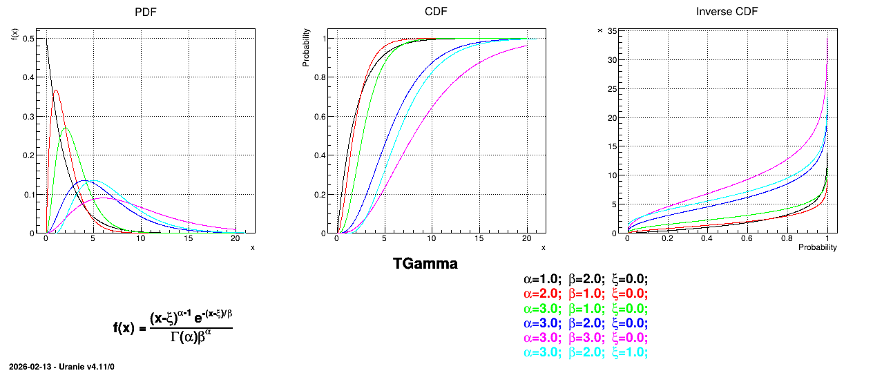

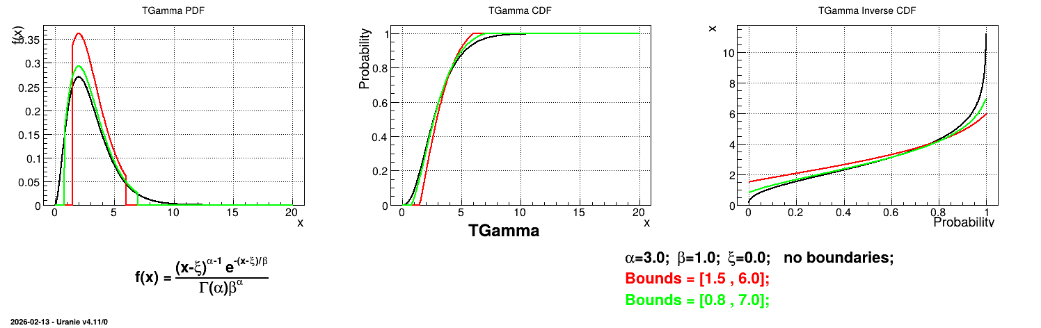
Is it also possible to set boundaries to the infinite span of this distribution to create a truncated Gamma law. This can be done by calling the following method:

tds.getAttribute("gam").setBounds(0.1,1.6)  # truncate the law

The resulting PDF, CDF and inverse CDF, with and without truncation, can be seen, in this case, in Figure 2.27 for a given set of parameters and various boundaries.