13.7.14. Macro “modelerTestKriging.py”
13.7.14.1. Objective
The idea is to provide a simple example of a kriging usage, and an how to, to produce plots in one dimension to represent the results. This example is the one taken from [Bla17] that uses a very simple set of six points as training database:
#TITLE: utf-1D-train.dat
#COLUMN_NAMES: x1|y

6.731290e-01 3.431918e-01
7.427596e-01 9.356860e-01
4.518467e-01 -3.499771e-01
2.215734e-02 2.400531e+00
9.915253e-01 2.412209e+00
1.815769e-01 1.589435e+00
The aim will be to get a kriging model that describes this dataset and to check its consistency over a certain number of points (here 100 points) which will be the testing database:
#TITLE: utf-1D-test.dat
#COLUMN_NAMES: x1|y

5.469435e-02 2.331524e+00
3.803054e-01 -3.277316e-02
7.047152e-01 6.030177e-01
2.360045e-02 2.398694e+00
9.271965e-01 2.268814e+00
7.868263e-01 1.324318e+00
7.791920e-01 1.257942e+00
6.107965e-01 -8.514510e-02
1.362316e-01 1.926999e+00
5.709913e-01 -2.758435e-01
8.738804e-01 1.992941e+00
2.251602e-01 1.219826e+00
9.175259e-01 2.228545e+00
5.128368e-01 -4.096161e-01
7.692913e-01 1.170999e+00
7.394406e-01 9.062407e-01
5.364506e-01 -3.772856e-01
1.861864e-01 1.551961e+00
7.573444e-01 1.065237e+00
1.005755e-01 2.141109e+00
9.114685e-01 2.201001e+00
3.628465e-01 7.920271e-02
2.383583e-01 1.103353e+00
7.468092e-01 9.716492e-01
3.126209e-01 4.578112e-01
8.034716e-01 1.466248e+00
6.730402e-01 3.424931e-01
8.021345e-01 1.455015e+00
2.503736e-01 9.966807e-01
9.001793e-01 2.145059e+00
7.019990e-01 5.799112e-01
6.001746e-01 -1.432102e-01
4.925013e-01 -4.126441e-01
5.685795e-01 -2.849419e-01
1.238257e-01 2.007351e+00
2.825838e-01 7.124861e-01
4.025708e-01 -1.574002e-01
8.562999e-01 1.875879e+00
3.214125e-01 3.865241e-01
2.021767e-01 1.418581e+00
6.338581e-01 5.717657e-02
3.042007e-01 5.276410e-01
4.860707e-01 -4.088007e-01
9.645326e-01 2.379243e+00
3.583711e-02 2.378513e+00
2.143110e-01 1.314473e+00
7.299624e-01 8.224203e-01
2.719263e-02 2.393622e+00
3.321495e-01 3.020224e-01
8.642671e-01 1.930341e+00
8.893604e-01 2.086039e+00
1.119469e-01 2.078562e+00
9.859741e-01 2.408725e+00
5.594688e-01 -3.166326e-01
1.904448e-01 1.516930e+00
4.232618e-01 -2.529865e-01
1.402221e-01 1.899932e+00
2.647519e-01 8.691058e-01
1.667035e-01 1.706823e+00
2.332246e-01 1.148786e+00
8.324190e-01 1.700059e+00
4.743443e-01 -3.958790e-01
3.435927e-01 2.154677e-01
9.846049e-01 2.407603e+00
9.705327e-01 2.390043e+00
6.631883e-01 2.662970e-01
6.153726e-01 -5.862472e-02
4.632361e-01 -3.766509e-01
6.474053e-01 1.502050e-01
7.161034e-02 2.273461e+00
4.514511e-01 -3.489255e-01
5.976782e-02 2.315661e+00
8.361934e-01 1.729000e+00
5.280981e-01 -3.922313e-01
9.394759e-01 2.313181e+00
2.710088e-01 8.138628e-01
8.161943e-01 1.571375e+00
5.047683e-01 -4.135789e-01
8.427635e-02 2.220534e+00
3.540224e-01 1.400987e-01
4.698548e-03 2.413597e+00
9.124315e-02 2.188105e+00
9.996285e-01 2.414210e+00
4.167139e-01 -2.249546e-01
5.892062e-01 -1.978247e-01
2.929336e-01 6.231119e-01
4.456454e-01 -3.325379e-01
1.148699e-02 2.410532e+00
3.892636e-01 -8.548741e-02
7.188374e-01 7.248622e-01
3.697949e-01 3.323350e-02
6.864519e-01 4.502113e-01
1.586679e-01 1.767741e+00
6.603030e-01 2.445009e-01
6.277168e-01 1.721489e-02
4.305704e-01 -2.817686e-01
1.553435e-01 1.792379e+00
5.476842e-01 -3.512131e-01
8.475444e-01 1.813503e+00
9.527370e-01 2.352313e+00
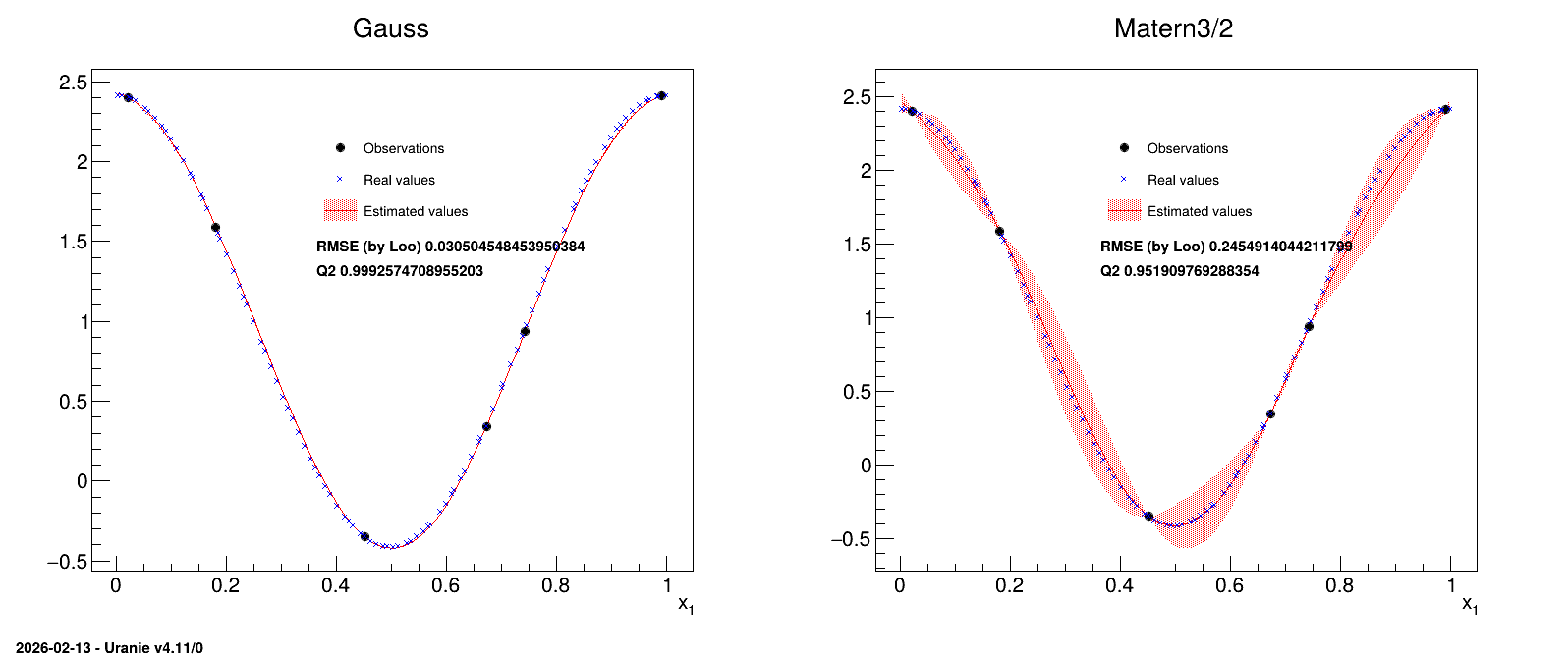
In this example, two different correlation functions are tested and the obtained results are compared at the end.
13.7.14.2. Macro Uranie
"""
Example of simple GP usage and illustration of results
"""
from math import sqrt
import numpy as np
from URANIE import DataServer, Modeler, Relauncher
import ROOT

def print_solutions(tds_obs, tds_estim, title):
    """Simple function to produce the 1D plot with observation
    points, testing points along with the uncertainty band."""

    nb_obs = tds_obs.getNPatterns()
    nb_est = tds_estim.getNPatterns()
    rx_arr = np.zeros([nb_est])
    x_arr = np.zeros([nb_est])
    y_est = np.zeros([nb_est])
    y_rea = np.zeros([nb_est])
    std_var = np.zeros([nb_est])

    tds_estim.computeRank("x1")
    tds_estim.getTuple().copyBranchData(rx_arr, nb_est, "Rk_x1")
    tds_estim.getTuple().copyBranchData(x_arr, nb_est, "x1")
    tds_estim.getTuple().copyBranchData(y_est, nb_est, "yEstim")
    tds_estim.getTuple().copyBranchData(y_rea, nb_est, "y")
    tds_estim.getTuple().copyBranchData(std_var, nb_est, "vEstim")

    xarr = np.zeros([nb_est])
    yest = np.zeros([nb_est])
    yrea = np.zeros([nb_est])
    stdvar = np.zeros([nb_est])

    for i in range(nb_est):
        ind = int(rx_arr[i]) - 1
        xarr[ind] = x_arr[i]
        yest[ind] = y_est[i]
        yrea[ind] = y_rea[i]
        stdvar[ind] = 2*sqrt(abs(std_var[i]))

    xobs = np.zeros([nb_obs])
    tds_obs.getTuple().copyBranchData(xobs, nb_obs, "x1")
    yobs = np.zeros([nb_obs])
    tds_obs.getTuple().copyBranchData(yobs, nb_obs, "y")

    gobs = ROOT.TGraph(nb_obs, xobs, yobs)
    gobs.SetMarkerColor(1)
    gobs.SetMarkerSize(1)
    gobs.SetMarkerStyle(8)
    zeros = np.zeros([nb_est])  # use doe plotting only
    gest = ROOT.TGraphErrors(nb_est, xarr, yest, zeros, stdvar)
    gest.SetLineColor(2)
    gest.SetLineWidth(1)
    gest.SetFillColor(2)
    gest.SetFillStyle(3002)
    grea = ROOT.TGraph(nb_est, xarr, yrea)
    grea.SetMarkerColor(4)
    grea.SetMarkerSize(1)
    grea.SetMarkerStyle(5)
    grea.SetTitle("Real Values")

    mgr = ROOT.TMultiGraph("toto", title)
    mgr.Add(gest, "l3")
    mgr.Add(gobs, "P")
    mgr.Add(grea, "P")
    mgr.Draw("A")
    mgr.GetXaxis().SetTitle("x_{1}")

    leg = ROOT.TLegend(0.4, 0.65, 0.65, 0.8)
    leg.AddEntry(gobs, "Observations", "p")
    leg.AddEntry(grea, "Real values", "p")
    leg.AddEntry(gest, "Estimated values", "lf")
    leg.Draw()
    return [mgr, leg]

# Create dataserver and read training database
tdsObs = DataServer.TDataServer("tdsObs", "observations")
tdsObs.fileDataRead("utf-1D-train.dat")
nbObs = 6

# Canvas, divided in 2
Can = ROOT.TCanvas("can", "can", 10, 32, 1600, 700)
apad = ROOT.TPad("apad", "apad", 0, 0.03, 1, 1)
apad.Draw()
apad.Divide(2, 1)

# Name of the plot and correlation functions used
outplot = "GaussAndMatern_1D_AllPoints.png"
Correl = ["Gauss", "Matern3/2"]

# Pointer to needed objects, created in the loop
gpb = [0, 0]
kg = [0, 0]
tdsEstim = [0, 0]
lkrig = [0, 0]

mgs = [0, 0]
legs = [0, 0]
# Looping over the two correlation function chosen
for im in range(2):

    # Create the TGPBuiler object with chosen option to find optimal parameters
    gpb[im] = Modeler.TGPBuilder(tdsObs, "x1", "y", Correl[im], "")
    gpb[im].findOptimalParameters("LOO", 100, "Subplexe", 1000)

    # Get the kriging object
    kg[im] = gpb[im].buildGP()

    # open the dataserver and read the testing basis
    tdsEstim[im] = DataServer.TDataServer("tdsEstim_"+str(im),
                                          "base de test")
    tdsEstim[im].fileDataRead("utf-1D-test.dat")

    # Applied resulting kriging on test basis
    lkrig[im] = Relauncher.TLauncher2(tdsEstim[im], kg[im], "x1",
                                      "yEstim:vEstim")
    lkrig[im].solverLoop()

    # do the plot
    apad.cd(im+1)
    mgs[im], legs[im] = print_solutions(tdsObs, tdsEstim[im], Correl[im])

    lat = ROOT.TLatex()
    lat.SetNDC()
    lat.SetTextSize(0.025)
    lat.DrawLatex(0.4, 0.61, "RMSE (by Loo) "+str(kg[im].getLooRMSE()))
    lat.DrawLatex(0.4, 0.57, "Q2 "+str(kg[im].getLooQ2()))
The first function of this macro (called PrintSolutions) is a complex part that will not be
detailed, used to represent the results.
The macro itself starts by reading the training database and storing it in a dataserver. A
TGPBuilder is created with the chosen correlation function and the hyper-parameters are estimation
by an optimisation procedure in:
gpb[im] = Modeler.TGPBuilder(tdsObs, "x1", "y", Correl[im], "")
gpb[im].findOptimalParameters("LOO", 100, "Subplexe", 1000)

kg[im] = gpb[im].buildGP()
The last line shows how to build and retrieve the newly created kriging object.
Finally, this kriging model is tested against the training database, thanks to a TLauncher2 object,
as following:
lkrig[im] = Relauncher.TLauncher2(tdsEstim[im], kg[im], "x1",
                                  "yEstim:vEstim")
lkrig[im].solverLoop()
13.7.14.3. Graph
Figure 13.45 Graph of the macro “modelerTestKriging.py”