13.11.3. Macro “calibrationLinBayesFlowrate1D.py”
13.11.3.1. Objective
The goal here is to calibrate the parameter \(H_l\) within the flowrate model, while varying only two
inputs (\(r_{\omega}\) and \(L\)). The remaining variables are fixed to the following values: \(r=25050\),
\(T_u=89335\), \(T_l=89.55\), \(H_u=1050\), \(K_{\omega}=10950\). The context of this example has already been
presented in Use-case for this chapter, including the model (implemented
here as a C++ function) and the initial lines defining the TDataServer objects. This macro demonstrates how
to apply a linear Bayesian estimation technique using a Relauncher-based architecture.
13.11.3.2. Macro Uranie
"""
Example of linear bayesian calibration with simple 1D flowrate model
"""
from URANIE import DataServer, Relauncher, Calibration
import ROOT

# Load the function flowrateCalib1D
ROOT.gROOT.LoadMacro("UserFunctions.C")

# Input reference file
ExpData = "Ex2DoE_n100_sd1.75.dat"

# define the reference
tdsRef = DataServer.TDataServer("tdsRef", "doe_exp_Re_Pr")
tdsRef.fileDataRead(ExpData)

# define the parameters
tdsPar = DataServer.TDataServer("tdsPar", "tdsPar")
tdsPar.addAttribute(DataServer.TUniformDistribution("hl", 700.0, 760.0))

# Create the output attribute
out = DataServer.TAttribute("out")

# Create interface to assessors
Reg = Relauncher.TCIntEval("flowrateModelnoH")
Reg.addInput(tdsRef.getAttribute("rw"))
Reg.addInput(tdsRef.getAttribute("l"))
Reg.addOutput(DataServer.TAttribute("H"))
runnoH = Relauncher.TSequentialRun(Reg)
runnoH.startSlave()
if runnoH.onMaster():
    launch = Relauncher.TLauncher2(tdsRef, runnoH)
    launch.solverLoop()
    runnoH.stopSlave()

# Create interface to assessors
Model = Relauncher.TCIntEval("flowrateCalib1D")
Model.addInput(tdsPar.getAttribute("hl"))
Model.addInput(tdsRef.getAttribute("rw"))
Model.addInput(tdsRef.getAttribute("l"))
Model.addOutput(out)

# Set the runner
runner = Relauncher.TSequentialRun(Model)

# Set the covariance matrix of the input reference
sd = tdsRef.getValue("sd_eps", 0)
mat = ROOT.TMatrixD(100, 100)
for ival in range(tdsRef.getNPatterns()):
    mat[ival][ival] = (sd*sd)

# Set the calibration object
cal = Calibration.TLinearBayesian(tdsPar, runner, 1, "")
cal.setLikelihood("gauss_lin", tdsRef, "rw:l", "Qexp")
cal.setObservationCovarianceMatrix(mat)
cal.setRegressorName("H")
cal.setParameterTransformationFunction(ROOT.transf)
cal.estimateParameters()

# Draw the parameters
canPar = ROOT.TCanvas("CanPar", "CanPar", 1200, 800)
padPar = ROOT.TPad("padPar", "padPar", 0, 0.03, 1, 1)
padPar.Draw()
padPar.cd()
cal.drawParameters("Parameters", "*", "nonewcanvas,transformed")

# Draw the residuals
canRes = ROOT.TCanvas("CanRes", "CanRes", 1200, 800)
padRes = ROOT.TPad("padRes", "padRes", 0, 0.03, 1, 1)
padRes.Draw()
padRes.cd()
cal.drawResiduals("Residuals", "*", "", "nonewcanvas")
Much of this code has already been covered in the previous section Macro “calibrationMinimisationFlowrate1D.py”
(up to the sequential run). The main difference here is that the input parameter is now defined as a
TStochasticDistribution, representing the a priori chosen distribution. In this example, it can
be either a TNormalDistribution or a TUniformDistribution (see [Bla17]), with the latter being
selected here:
tdsPar.addAttribute(DataServer.TUniformDistribution("hl", 700.0, 760.0))
Another difference from the previous example is that the method must be slightly adapted to obtain values
for the regressor. As discussed in [Bla17], linear Bayesian estimation can be applied when the model is
approximately linear. This requires linearising the flowrate function, as demonstrated here:
Here, the regressor can be expressed as
From this expression, it is clear that we will be calibrating a newly defined parameter
\(\theta = \left( H_u - H_l\right)\), which must later be converted back into the parameter of interest. To
obtain the regressor estimation, we simply use another C++ function, flowrateModelnoH, together with the
standard Relauncher approach:
# Create interface to assessors
Reg = Relauncher.TCIntEval("flowrateModelnoH")
Reg.addInput(tdsRef.getAttribute("rw"))
Reg.addInput(tdsRef.getAttribute("l"))
Reg.addOutput(DataServer.TAttribute("H"))
runnoH = Relauncher.TSequentialRun(Reg)
runnoH.startSlave()
if runnoH.onMaster():
    launch = Relauncher.TLauncher2(tdsRef, runnoH)
    launch.solverLoop()
    runnoH.stopSlave()
This method also requires the input covariance matrix. The provided dataset (Ex2DoE_n100_sd1.75.dat) contains
an estimate of the uncertainty affecting the reference measurements. Since this uncertainty is constant across
all samples, the input covariance matrix is diagonal, with each diagonal element equal to the square of the
standard deviation, as illustrated below:
# Set the covariance matrix of the input reference
sd = tdsRef.getValue("sd_eps", 0)
mat = ROOT.TMatrixD(100, 100)
for ival in range(tdsRef.getNPatterns()):
    mat[ival][ival] = (sd*sd)
The model is defined (from a TCIntEval instance with the three input variables discussed above,
in the correct order) along with the computation distribution method (sequential).
The calibration object is then created using a Mahalanobis distance function, which is used here for illustrative purposes (see Analytical linear Bayesian estimation for more details). The three key steps are:
Providing the input covariance matrix via the
setObservationCovarianceMatrixmethod;Specifying the regressors’ names using
setRegressorName;Defining the parameter transformation function (optional) with
setParameterTransformationFunction.
The final step is more involved: since we are calibrating \(\theta\), we need to recover the corresponding parameter
value at the end. This is achieved by providing a C++ function that transforms the parameter estimated from the
linearisation back into the parameter of interest. For illustration, this is implemented in UserFunctions.C via
the transf function, shown below:
void transf(double *x, double *res)
{
    res[0] = 1050 - x[0];  // simply H_l = \theta - H_u
}
The complete block of code discussed in this section is as follows:
# Set the calibration object
cal = Calibration.TLinearBayesian(tdsPar, runner, 1, "")
cal.setLikelihood("gauss_lin", tdsRef, "rw:l", "Qexp")
cal.setObservationCovarianceMatrix(mat)
cal.setRegressorName("H")
cal.setParameterTransformationFunction(ROOT.transf)
cal.estimateParameters()
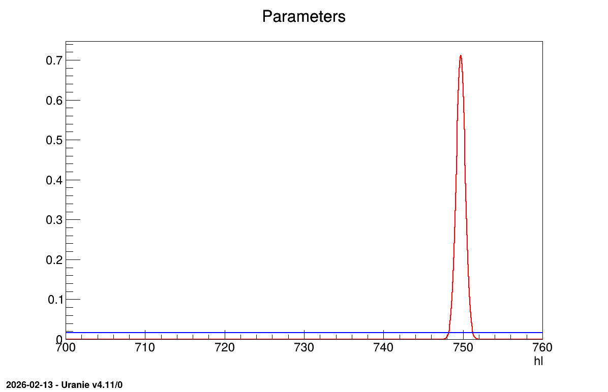
The final part demonstrates how to display the results. Since this method produces normal a posteriori distributions, they are represented by a vector of means and a covariance structure, both easily accessible. The means are displayed on screen, as illustrated in Console. Two additional pieces of a posteriori information are presented as plots: the residuals (Figure 13.62), which show the expected normal distribution behavior, as discussed in [Bla17] and the posterior distribution (Figure 13.63).
# Draw the parameters
canPar = ROOT.TCanvas("CanPar", "CanPar", 1200, 800)
padPar = ROOT.TPad("padPar", "padPar", 0, 0.03, 1, 1)
padPar.Draw()
padPar.cd()
cal.drawParameters("Parameters", "*", "nonewcanvas,transformed")

# Draw the residuals
canRes = ROOT.TCanvas("CanRes", "CanRes", 1200, 800)
padRes = ROOT.TPad("padRes", "padRes", 0, 0.03, 1, 1)
padRes.Draw()
padRes.cd()
cal.drawResiduals("Residuals", "*", "", "nonewcanvas")
13.11.3.3. Console
--- Uranie v4.11/0 --- Developed with ROOT (6.36.06)
                      Copyright (C) 2013-2026 CEA/DES
                      Contact: support-uranie@cea.fr
                      Date: Thu Feb 12, 2026

***  TLinearBayesian::computeParameters(); Transformed parameters estimated are

1x1 matrix is as follows

     |      0    |
------------------
   0 |      749.7
13.11.3.4. Graphs
Figure 13.62 Residuals graph of the macro “calibrationLinBayesFlowrate1D.py”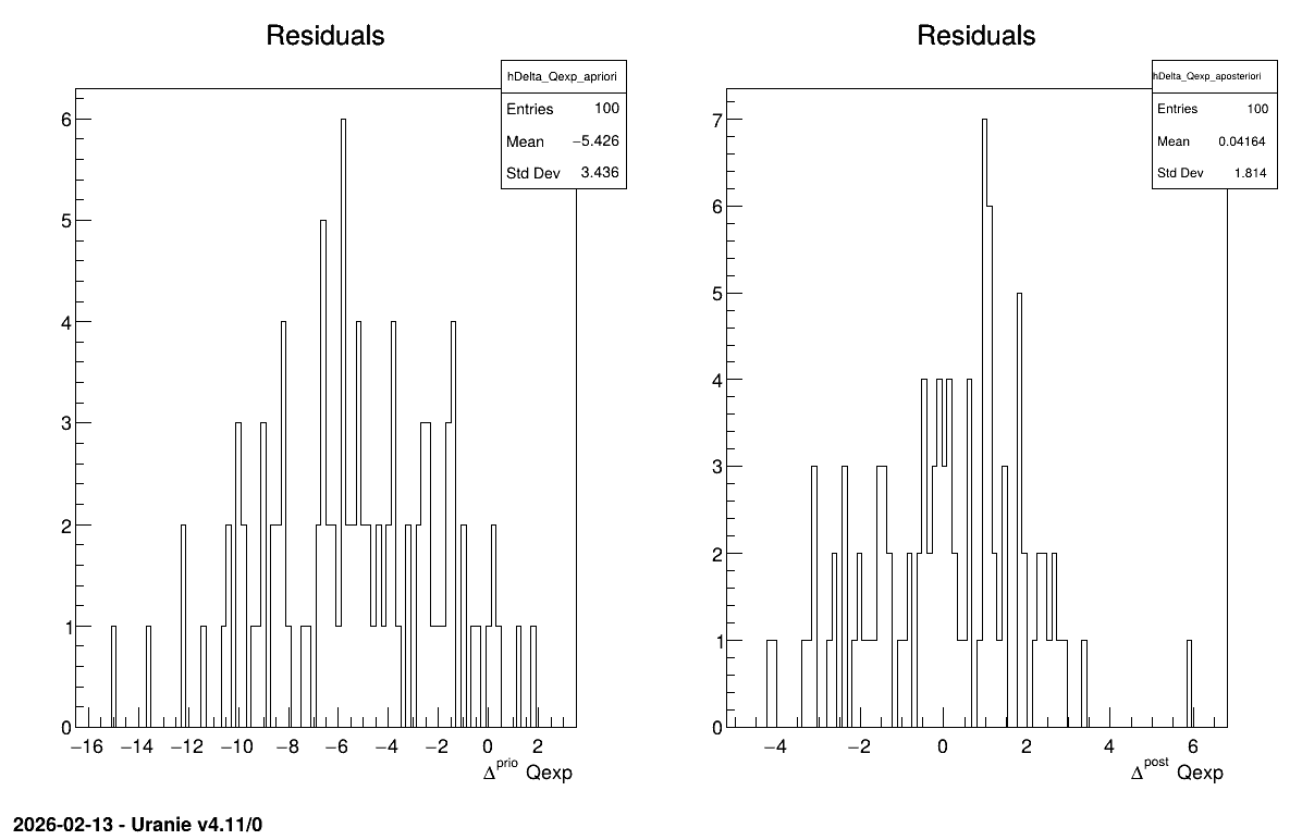
Figure 13.63 Parameter graph of the macro “calibrationLinBayesFlowrate1D.py”