13.11.2. Macro “calibrationMinimisationFlowrate2DVizir.py”
13.11.2.1. Objective
The goal here is to calibrate the parameters \(H_u\) and \(H_l\) within the flowrateCalib2D model
(a two-dimensional version of the flowrate model), while varying only two inputs (\(r_{\omega}\)
and \(L\)). The remaining variables are fixed to the following values: \(r=25050\), \(T_u=89335\),
\(T_l=89.55\), \(K_{\omega}=10950\). The context of this example has already been presented in
Use-case for this chapter, including the model (implemented
here as a C++ function) and the initial lines defining the TDataServer objects.
In addition to what has been presented in Macro “calibrationMinimisationFlowrate1D.py”, this macro introduces two new elements:
the use of Vizir instead of a simpler
TNloptSolver-inheriting instance;the discussion of problem identifiability, as introduced in [Bla17].
13.11.2.2. Macro Uranie
"""
Example of calibration through minimisation with Vizir in Flowrate 2D
"""
from URANIE import DataServer, Relauncher, Reoptimizer, Calibration
import ROOT
# Load the function flowrateCalib2DVizir
ROOT.gROOT.LoadMacro("UserFunctions.C")

# Input reference file
ExpData = "Ex2DoE_n100_sd1.75.dat"

# define the reference
tdsRef = DataServer.TDataServer("tdsRef", "doe_exp_Re_Pr")
tdsRef.fileDataRead(ExpData)

# define the parameters
tdsPar = DataServer.TDataServer("tdsPar", "tdsPar")
tdsPar.addAttribute(DataServer.TAttribute("hu", 1020.0, 1080.0))
tdsPar.addAttribute(DataServer.TAttribute("hl", 720.0, 780.0))

# Create the output attribute
out = DataServer.TAttribute("out")

# Create interface to assessors
Model = Relauncher.TCIntEval("flowrateCalib2D")
Model.addInput(tdsPar.getAttribute("hu"))
Model.addInput(tdsPar.getAttribute("hl"))
Model.addInput(tdsRef.getAttribute("rw"))
Model.addInput(tdsRef.getAttribute("l"))
Model.addOutput(out)

# Set the runner
runner = Relauncher.TSequentialRun(Model)

# Set the calibration object
cal = Calibration.TMinimisation(tdsPar, runner, 1)
cal.setDistance("relativeLS", tdsRef, "rw:l", "Qexp")
# Set optimisaiton properties
solv = Reoptimizer.TVizirGenetic()
solv.setSize(24, 15000, 100)
cal.setOptimProperties(solv)
# cal.getOptimMaster().setTolerance(1e-6)
cal.estimateParameters()

# Draw the residuals
canRes = ROOT.TCanvas("CanRes", "CanRes", 1200, 800)
padRes = ROOT.TPad("padRes", "padRes", 0, 0.03, 1, 1)
padRes.Draw()
padRes.cd()
cal.drawResiduals("Residuals", "*", "", "nonewcanvas")

# Draw the box plot of parameters
canPar = ROOT.TCanvas("CanPar", "CanPar", 1200, 800)
tdsPar.getTuple().SetMarkerStyle(20)
tdsPar.getTuple().SetMarkerSize(0.8)
tdsPar.Draw("hu:hl")

# Look at the correlation and statistic
tdsPar.computeStatistic("hu:hl")
corr = tdsPar.computeCorrelationMatrix("hu:hl")
corr.Print()

print("hl is %3.8g +- %3.8g " % (tdsPar.getAttribute("hl").getMean(),
                                 tdsPar.getAttribute("hl").getStd()))
print("hu is %3.8g +- %3.8g " % (tdsPar.getAttribute("hu").getMean(),
                                 tdsPar.getAttribute("hu").getStd()))
Much of this code has already been covered in the previous section
Macro “calibrationMinimisationFlowrate1D.py” (up to the sequential run). The main
difference here is that the input parameter is now defined as a TAttribute with boundaries
specifying the space in which the algorithm will search.
tdsPar.addAttribute(DataServer.TAttribute("hu", 1020.0, 1080.0))
tdsPar.addAttribute(DataServer.TAttribute("hl", 720.0, 780.0))
The model is defined (from a TCIntEval instance with the three input variables discussed above,
in the correct order) along with the computation distribution method (sequential).
# Create interface to assessors
Model = Relauncher.TCIntEval("flowrateCalib2D")
Model.addInput(tdsPar.getAttribute("hu"))
Model.addInput(tdsPar.getAttribute("hl"))
Model.addInput(tdsRef.getAttribute("rw"))
Model.addInput(tdsRef.getAttribute("l"))
Model.addOutput(out)

# Set the runner
runner = Relauncher.TSequentialRun(Model)
Once this setup is complete, the calibration object (TMinimisation) is created. As explained in
Recommended distance and likelihood functions, construction method, the first step is
to define the distance function (here the relative least squares distance) using setDistance. This method
also specifies the TDataServer containing the reference data, the names of the reference inputs, and the reference
variable against which the model output is compared. Finally, the optimisation algorithm is defined by creating
an instance of TVizirGenetic, and the parameters are then estimated.
# Set the calibration object
cal = Calibration.TMinimisation(tdsPar, runner, 1)
cal.setDistance("relativeLS", tdsRef, "rw:l", "Qexp")
# Set optimisaiton properties
solv = Reoptimizer.TVizirGenetic()
solv.setSize(24, 15000, 100)
cal.setOptimProperties(solv)
# cal.getOptimMaster().setTolerance(1e-6)
cal.estimateParameters()
The final part demonstrates how to display the results. Since this method produces a point estimate, only a
single value is obtained, which is always shown on the screen, as illustrated in
Console. Another important aspect is to examine the residuals,
as discussed in [Bla17]. This is illustrated in Figure 13.60, which
shows the residuals of the a posteriori estimates, typically following a normal
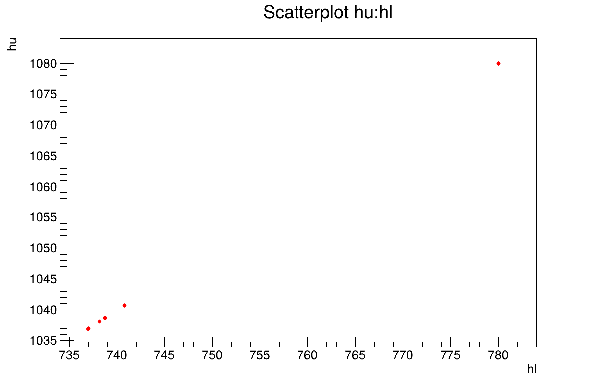
distribution. Finally, the parameter graph (Figure 13.61)
reveals a wide variety of possible solutions. This highlights a problem of identifiability,
since infinitely many parameter combinations can lead to the same results, as further confirmed
by the correlation matrix shown in Console.
# Draw the residuals
canRes = ROOT.TCanvas("CanRes", "CanRes", 1200, 800)
padRes = ROOT.TPad("padRes", "padRes", 0, 0.03, 1, 1)
padRes.Draw()
padRes.cd()
cal.drawResiduals("Residuals", "*", "", "nonewcanvas")

# Draw the box plot of parameters
canPar = ROOT.TCanvas("CanPar", "CanPar", 1200, 800)
tdsPar.getTuple().SetMarkerStyle(20)
tdsPar.getTuple().SetMarkerSize(0.8)
tdsPar.Draw("hu:hl")

# Look at the correlation and statistic
tdsPar.computeStatistic("hu:hl")
corr = tdsPar.computeCorrelationMatrix("hu:hl")
corr.Print()

print("hl is %3.8g +- %3.8g " % (tdsPar.getAttribute("hl").getMean(),
                                 tdsPar.getAttribute("hl").getStd()))
print("hu is %3.8g +- %3.8g " % (tdsPar.getAttribute("hu").getMean(),
                                 tdsPar.getAttribute("hu").getStd()))
13.11.2.3. Console
--- Uranie v4.11/0 --- Developed with ROOT (6.36.06)
                      Copyright (C) 2013-2026 CEA/DES
                      Contact: support-uranie@cea.fr
                      Date: Thu Feb 12, 2026

first 100
Genetic  1

  Generation : 1, rang max 23
	Nb d'evaluation : 100, taille de la Z.P. :  0

  Generation : 2, rang max 23
	Nb d'evaluation : 465, taille de la Z.P. :  1

  Generation : 3, rang max 8
	Nb d'evaluation : 963, taille de la Z.P. :  6

  Generation : 4, rang max 0
	Nb d'evaluation : 1617, taille de la Z.P. :  24
Genetic  converge 1617
************************************************************************************
*    Row   * tdsPar__n *     hu.hu *     hl.hl * agreement * rgpareto. * generatio *
************************************************************************************
*        0 *         0 * 1038.1302 * 738.13383 * 0.3639076 *         0 *         3 *
*        1 *         1 *      1080 *       780 * 0.3639083 *         0 *         3 *
*        2 *         2 * 1040.7058 * 740.77116 * 0.3639018 *         0 *         3 *
*        3 *         3 * 1079.9545 *       780 * 0.3639024 *         0 *         3 *
*        4 *         4 * 1040.7058 * 740.77116 * 0.3639018 *         0 *         1 *
*        5 *         5 * 1038.6638 * 738.70819 * 0.3639025 *         0 *         3 *
*        6 *         6 * 1040.7058 * 740.77116 * 0.3639018 *         0 *         3 *
*        7 *         7 * 1036.9776 * 736.98122 * 0.3639076 *         0 *         3 *
*        8 *         8 * 1036.9776 * 736.98122 * 0.3639076 *         0 *         3 *
*        9 *         9 * 1038.6638 * 738.70819 * 0.3639025 *         0 *         3 *
*       10 *        10 * 1036.9776 * 736.98122 * 0.3639076 *         0 *         2 *
*       11 *        11 *      1080 *       780 * 0.3639083 *         0 *         3 *
*       12 *        12 * 1036.9776 * 736.98122 * 0.3639076 *         0 *         3 *
*       13 *        13 * 1040.7058 * 740.77116 * 0.3639018 *         0 *         2 *
*       14 *        14 *      1080 *       780 * 0.3639083 *         0 *         3 *
*       15 *        15 *      1080 *       780 * 0.3639083 *         0 *         3 *
*       16 *        16 * 1038.6638 * 738.70819 * 0.3639025 *         0 *         3 *
*       17 *        17 * 1040.7058 * 740.77116 * 0.3639018 *         0 *         3 *
*       18 *        18 *      1080 *       780 * 0.3639083 *         0 *         3 *
*       19 *        19 * 1036.9776 * 736.98122 * 0.3639076 *         0 *         3 *
*       20 *        20 * 1036.9042 * 736.96108 * 0.3639019 *         0 *         3 *
*       21 *        21 * 1038.6638 * 738.70819 * 0.3639025 *         0 *         3 *
*       22 *        22 *      1080 *       780 * 0.3639083 *         0 *         3 *
*       23 *        23 *      1080 *       780 * 0.3639083 *         0 *         3 *
************************************************************************************

2x2 matrix is as follows

     |      0    |      1    |
-------------------------------
   0 |          1           1
   1 |          1           1

hl is 752.4454 +- 19.946252
hu is 1052.4192 +- 19.959796
13.11.2.4. Graphs
Figure 13.60 Residuals graph of the macro “calibrationMinimisationFlowrate2DVizir.py”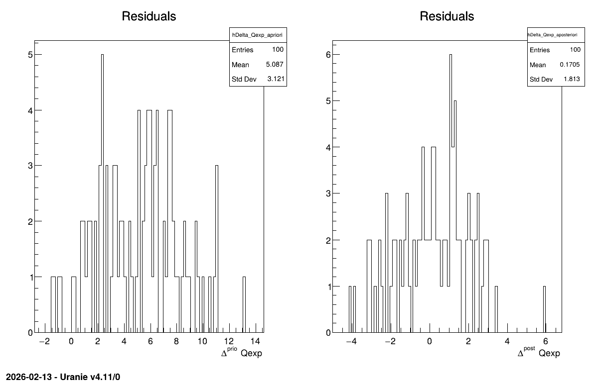
Figure 13.61 Parameter graph of the macro “calibrationMinimisationFlowrate2DVizir.py”