13.11.4. Macro “calibrationRejectionABCFlowrate1D.py”

13.11.4.1. Objective

The goal here is to calibrate the parameter \(H_l\) within the flowrate model, while varying only two inputs (\(r_{\omega}\) and \(L\)). The remaining variables are fixed to the following values: \(r=25050\), \(T_u=89335\), \(T_l=89.55\), \(H_u=1050\), \(K_{\omega}=10950\). The context of this example has already been presented in Use-case for this chapter, including the model (implemented here as a C++ function) and the initial lines defining the TDataServer objects. This macro demonstrates how to apply a rejection ABC method using a Relauncher-based architecture.

13.11.4.2. Macro Uranie

"""
Example of calibration using Rejection ABC approach on flowrate 1D
"""
from URANIE import DataServer, Calibration, Relauncher
import ROOT

# Load the function flowrateCalib1D
ROOT.gROOT.LoadMacro("UserFunctions.C")

# Input reference file
ExpData = "Ex2DoE_n100_sd1.75.dat"

# define the reference
tdsRef = DataServer.TDataServer("tdsRef", "doe_exp_Re_Pr")
tdsRef.fileDataRead(ExpData)

# define the parameters
tdsPar = DataServer.TDataServer("tdsPar", "tdsPar")
tdsPar.addAttribute(DataServer.TUniformDistribution("hl", 700.0, 760.0))

# Create the output attribute
out = DataServer.TAttribute("out")

# Create interface to assessors
Model = Relauncher.TCIntEval("flowrateCalib1D")
Model.addInput(tdsPar.getAttribute("hl"))
Model.addInput(tdsRef.getAttribute("rw"))
Model.addInput(tdsRef.getAttribute("l"))
Model.addOutput(out)

# Set the runner
runner = Relauncher.TSequentialRun(Model)

# Set the calibration object
nABC = 100
eps = 0.05
cal = Calibration.TRejectionABC(tdsPar, runner, nABC, "")
cal.setDistance("LS", tdsRef, "rw:l", "Qexp")
cal.setGaussianNoise("sd_eps")
cal.setPercentile(eps)
cal.estimateParameters()

# Draw the parameters
canPar = ROOT.TCanvas("CanPar", "CanPar", 1200, 800)
padPar = ROOT.TPad("padPar", "padPar", 0, 0.03, 1, 1)
padPar.Draw()
padPar.cd()
cal.drawParameters("Parameters", "*", "nonewcanvas")

# Draw the residuals
canRes = ROOT.TCanvas("CanRes", "CanRes", 1200, 800)
padRes = ROOT.TPad("padRes", "padRes", 0, 0.03, 1, 1)
padRes.Draw()
padRes.cd()
cal.drawResiduals("Residuals", "*", "", "nonewcanvas")

# Compute statistics
tdsPar.computeStatistic()
print("The mean of hl is %3.8g" % (tdsPar.getAttribute("hl").getMean()))
print("The std of hl is %3.8g" % (tdsPar.getAttribute("hl").getStd()))

Much of this code has already been covered in the previous section Macro “calibrationMinimisationFlowrate1D.py” (up to the sequential run). The main difference here is that the input parameter is now defined as a TStochasticDistribution, representing the a priori chosen distribution.

tdsPar.addAttribute(DataServer.TUniformDistribution("hl", 700.0, 760.0))

The model is defined (from a TCIntEval instance with the three input variables discussed above, in the correct order) along with the computation distribution method (sequential).

The calibration object is then created by specifying both the number of elements in the final sample (nABC = 100) and the percentile of events retained (eps = 0.05, meaning that 2000 locations will be tested). Since the code is deterministic, uncertainty is introduced by adding random Gaussian noise. The standard deviation of this noise is defined on an event-by-event basis using a variable from the observation dataserver. Finally, the distance function is specified, and the estimation process is performed.

# Set the calibration object
nABC = 100
eps = 0.05
cal = Calibration.TRejectionABC(tdsPar, runner, nABC, "")
cal.setDistance("LS", tdsRef, "rw:l", "Qexp")
cal.setGaussianNoise("sd_eps")
cal.setPercentile(eps)
cal.estimateParameters()

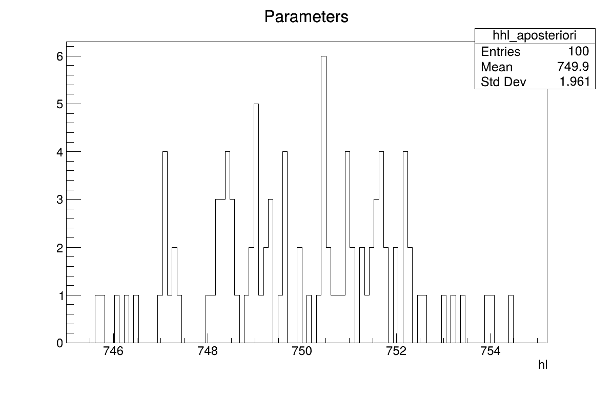
The final part demonstrates how to display the results. Since this method produces samples of the a posteriori distributions, basic statistical information are directly displayed on screen, as shown in Console. Two additional pieces of a posteriori information are presented as plots: the residuals (Figure 13.64), which show the expected normal distribution behavior, as discussed in [Bla17] and the posterior distribution (Figure 13.65).

# Draw the parameters
canPar = ROOT.TCanvas("CanPar", "CanPar", 1200, 800)
padPar = ROOT.TPad("padPar", "padPar", 0, 0.03, 1, 1)
padPar.Draw()
padPar.cd()
cal.drawParameters("Parameters", "*", "nonewcanvas")

# Draw the residuals
canRes = ROOT.TCanvas("CanRes", "CanRes", 1200, 800)
padRes = ROOT.TPad("padRes", "padRes", 0, 0.03, 1, 1)
padRes.Draw()
padRes.cd()
cal.drawResiduals("Residuals", "*", "", "nonewcanvas")

# Compute statistics
tdsPar.computeStatistic()
print("The mean of hl is %3.8g" % (tdsPar.getAttribute("hl").getMean()))
print("The std of hl is %3.8g" % (tdsPar.getAttribute("hl").getStd()))

13.11.4.3. Console

--- Uranie v4.11/0 --- Developed with ROOT (6.36.06)
                      Copyright (C) 2013-2026 CEA/DES 
                      Contact: support-uranie@cea.fr 
                      Date: Thu Feb 12, 2026

 <URANIE::INFO> 
 <URANIE::INFO> *** URANIE INFORMATION ***
 <URANIE::INFO> *** File[${SOURCEDIR}/meTIER/calibration/souRCE/TDistanceLikelihoodFunction.cxx] Line[601]
 <URANIE::INFO> TDistanceLikelihoodFunction::setGaussianRandomNoise: gaussian random noise(s) is added using information in [sd_eps] to modify the output variable(s) [out]. 
 <URANIE::INFO> *** END of URANIE INFORMATION ***
 <URANIE::INFO> 
 <URANIE::INFO> 
 <URANIE::INFO> *** URANIE INFORMATION ***
 <URANIE::INFO> *** File[${SOURCEDIR}/meTIER/calibration/souRCE/TRejectionABC.cxx] Line[118]
 <URANIE::INFO> TRejectionABC::computeParameters:: 2000 evaluations will be performed ! 
 <URANIE::INFO> *** END of URANIE INFORMATION ***
 <URANIE::INFO> 
A posteriori mean coordinates are : (749.926)
The mean of hl is 749.92609
The std of hl is 1.9704229

13.11.4.4. Graphs

../../_images/calibrationRejectionABCFlowrate1D_Res.png — Figure 13.64 Residuals graph of the macro **“calibrationRejectionABCFlowrate1D.py”**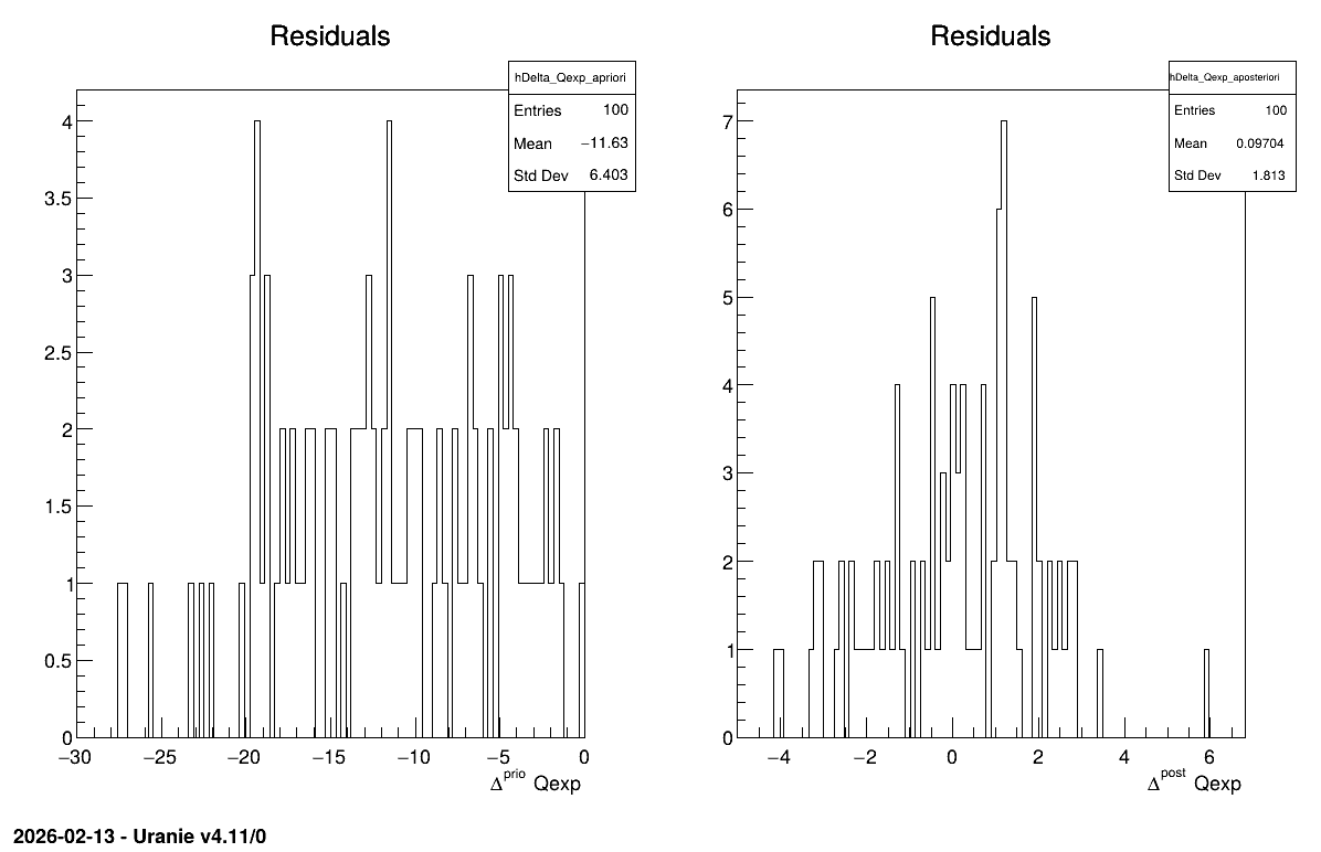

../../_images/calibrationRejectionABCFlowrate1D_Par.png — Figure 13.65 Parameter graph of the macro **“calibrationRejectionABCFlowrate1D.py”**