13.11.6. Macro “calibrationMCMCLinReg.py”
13.11.6.1. Objective
The goal here is to calibrate the parameters \(t_0\) (constant term) and \(t_1\) (multiplicative term)
within a simple linear model (implemented in UserFunctions.C), against the observable
outputs \(y_{Exp}\), associated with given values of \(x\) stored in the input file linReg_Database.dat.
The initial lines defining the TDataServer and the model are similar to those presented in
Use-case for this chapter. This macro demonstrates how to apply
the Markov chain Monte Carlo approach and more precisely the classic Metropolis-Hastings
algorithm in two dimensions using a Relauncher-based architecture.
13.11.6.2. Macro Uranie
"""
Example of calibration using MCMC algo on linear model
"""
from URANIE import DataServer, Relauncher, Calibration
import ROOT

# Load the function Toy
ROOT.gROOT.LoadMacro("UserFunctions.C")

# Input reference file
ExpData = "linReg_Database.dat"

# Define the reference
tdsRef = DataServer.TDataServer("tdsRef", "doe_exp_Re_Pr")
tdsRef.fileDataRead(ExpData)

# Define the uncertainty model guessing the standard deviation (here 0.2)
tdsRef.addAttribute("sd_eps", "0.2")

# Define the parameters
tdsPar = DataServer.TDataServer("tdsPar", "tdsPar")
binf_sea = -2.0
bsup_sea = 2.0
tdsPar.addAttribute(DataServer.TUniformDistribution("t0", binf_sea, bsup_sea))
tdsPar.addAttribute(DataServer.TUniformDistribution("t1", binf_sea, bsup_sea))

# Create the output attribute
out = DataServer.TAttribute("out")

# Create interface to assessors
myeval = Relauncher.TCIntEval("Toy")
myeval.addInput(tdsRef.getAttribute("x"))
myeval.addInput(tdsPar.getAttribute("t0"))
myeval.addInput(tdsPar.getAttribute("t1"))
myeval.addOutput(out)

# Set the runner
run = Relauncher.TSequentialRun(myeval)

# Set the calibration object with default Metropolis-Hastings algorithm
cal = Calibration.TMCMC(tdsPar, run, 4000)

# Set the likelihood and reference with default gaussian log likelihood
cal.setLikelihood("log-gauss", tdsRef, "x", "yExp", "sd_eps")

# Set the number of iterations between two information displays
cal.setNbDump(1000)

# Initialise 4 chains
cal.setMultistart(4)

# Set the starting points of each chain
cal.setStartingPoints(0, [0.5, -0.2])
cal.setStartingPoints(1, [-1.5, 1])
cal.setStartingPoints(2, [-1.2, -0.2])
cal.setStartingPoints(3, [0.3, 0.8])

# Set the standard deviation of the proposal for all the chains
cal.setProposalStd(-1, [0.05, 0.05])

# Run the MCMC algorithm
cal.estimateParameters()

# Quality assessment: Draw the trace of the Markov Chain
canTr = ROOT.TCanvas("CanTr", "CanTr", 1200, 800)
padTr = ROOT.TPad("padTr", "padTr", 0, 0.03, 1, 1)
padTr.Draw()
padTr.cd()
cal.drawTrace("Trace", "*", "nonewcanvas")

# Quality assessment: Draw the acceptation ratio
canAcc = ROOT.TCanvas("CanAcc", "CanAcc", 1200, 800)
padAcc = ROOT.TPad("padAcc", "padAcc", 0, 0.03, 1, 1)
padAcc.Draw()
padAcc.cd()
cal.drawAcceptationRatio("Acceptation ratio", "*", "nonewcanvas")

# Set the number of iterations to remove
burnin = 100
cal.setBurnin(burnin)

# Verify that the burn-in has been set correctely with Gelman-Rubin statistic
GelmanRubin_values = cal.diagGelmanRubin()

# Compute Effective Sample Size
ESS_values = cal.diagESS()

# Set the lag
lag = 3
cal.setLag(lag)

# Quality assessment: Draw the 2D trace of the Markov Chain
canTr2D = ROOT.TCanvas("CanTr2D", "CanTr2D", 1200, 800)
padTr2D = ROOT.TPad("padTr2D", "padTr2D", 0, 0.03, 1, 1)
padTr2D.Draw()
padTr2D.cd()
cal.draw2DTrace("Trace 2D", "t0:t1", "nonewcanvas")

# Draw the residuals
canRes = ROOT.TCanvas("CanRes", "CanRes", 1200, 800)
padRes = ROOT.TPad("padRes", "padRes", 0, 0.03, 1, 1)
padRes.Draw()
padRes.cd()
cal.drawResiduals("Residuals", "*", "", "nonewcanvas")

# Draw the posterior distributions
canPar = ROOT.TCanvas("CanPar","CanPar",1200,800)
padPar = ROOT.TPad("padPar","padPar",0, 0.03, 1, 1)
padPar.Draw()
padPar.cd()
cal.drawParameters("Posterior", "*", "nonewcanvas")
Much of this code has already been covered in the previous section
Macro “calibrationMinimisationFlowrate1D.py” (up to the sequential run). The main difference here
is that the input parameter is now defined as a TStochasticDistribution, representing the a priori
chosen distribution.
Another difference from the previous example Macro “calibrationMCMCFlowrate1D.py” is that no uncertainty associated with the observables is provided in the input file. To this end, a new attribute is defined and added to the reference dataserver, with an assumed standard deviation of \(y_{Exp}\) equal to 0.2.
# Define the uncertainty model guessing the standard deviation (here 0.2)
tdsRef.addAttribute("sd_eps", "0.2")

# Define the parameters
tdsPar = DataServer.TDataServer("tdsPar", "tdsPar")
binf_sea = -2.0
bsup_sea = 2.0
tdsPar.addAttribute(DataServer.TUniformDistribution("t0", binf_sea, bsup_sea))
tdsPar.addAttribute(DataServer.TUniformDistribution("t1", binf_sea, bsup_sea))
The model is defined (from a TCIntEval instance with the three input variables discussed above,
in the correct order) along with the computation distribution method (sequential).
The calibration object is then created by specifying both the number of iterations of the algorithm (set to 4000). The likelihood function is defined as Gaussian, with the reference dataserver, the input and output variables, and the assumed standard deviation of the experimental data (see previous paragraph) provided as arguments. Several additional options are configured: the interval between two console displays is specified, the number of chains to initialise is defined, the starting points of each chain are assigned (one by one), and the standard deviation of the initial proposal distribution is set (for all chains at once). For further details on these options, see Defining the TMCMC properties. Finally, the estimation process is performed, using the default MCMC algorithm (classic Metropolis-Hastings).
# Set the calibration object with default Metropolis-Hastings algorithm
cal = Calibration.TMCMC(tdsPar, run, 4000)

# Set the likelihood and reference with default gaussian log likelihood
cal.setLikelihood("log-gauss", tdsRef, "x", "yExp", "sd_eps")

# Set the number of iterations between two information displays
cal.setNbDump(1000)

# Initialise 4 chains
cal.setMultistart(4)

# Set the starting points of each chain
cal.setStartingPoints(0, [0.5, -0.2])
cal.setStartingPoints(1, [-1.5, 1])
cal.setStartingPoints(2, [-1.2, -0.2])
cal.setStartingPoints(3, [0.3, 0.8])

# Set the standard deviation of the proposal for all the chains
cal.setProposalStd(-1, [0.05, 0.05])

# Run the MCMC algorithm
cal.estimateParameters()
The final part demonstrates how to display and analyse the results. The first elements to examine are the trace plot (Figure 13.70) and the acceptance ratio plot (Figure 13.71). On these plots, you should check that the number of accepted iterations is sufficiently high (at least several hundred if the chains stabilise quickly — in our case, around 1500), and that the converged acceptance ratio falls within a reasonable range (20–50% — here, it is close to 40%). When inspecting the trace, the chains should have converged around the same region (as they do here), and they should evolve rapidly, which indicates efficient exploration and low autocorrelation (also observed in our case). Finally, these plots help verify whether all chains behave stably and from which iteration they can be considered stable. This provides a first indication of a suitable burn-in value. In this example, the chains appear to have converged, and a burn-in value of 100 seems appropriate.
The burn-in size can then be defined and its consistency verified using the Gelman–Rubin statistic. In our case, values of 1.00092 and 0.99993 (for parameters \(t_0\) and \(t_1\) respectively) are reported in Console which are very close to 1 and confirms excellent convergence of the chains for both parameters. Otherwise, a different burn-in value might have been more appropriate, the calculation could have been extended, or the MCMC algorithm settings adjusted.
The next step is to check for sample autocorrelation within the chains. The Effective Sample Size (ESS) provides a good indication of the lag to be used. In our case, the chains contain a reasonable number of independent samples (at least 424 each), and a lag of 3 is sufficient (see Console). Otherwise, the calculation could have been extended, or the MCMC algorithm settings adjusted (especially the standard deviation of the proposal distribution).
It is also possible to represent the chains in two dimensions (Figure 13.72). This provides an alternative way to verify whether the chains converge to the same region and highlights potential covariance between the posterior distributions of the two parameters.
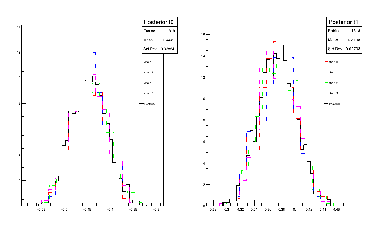
Two additional pieces of a posteriori information are presented as plots: the residuals (Figure 13.73), which show the expected normal distribution behavior, as discussed in [Bla17] and the posterior distribution (Figure 13.74).
# Quality assessment: Draw the trace of the Markov Chain
canTr = ROOT.TCanvas("CanTr", "CanTr", 1200, 800)
padTr = ROOT.TPad("padTr", "padTr", 0, 0.03, 1, 1)
padTr.Draw()
padTr.cd()
cal.drawTrace("Trace", "*", "nonewcanvas")

# Quality assessment: Draw the acceptation ratio
canAcc = ROOT.TCanvas("CanAcc", "CanAcc", 1200, 800)
padAcc = ROOT.TPad("padAcc", "padAcc", 0, 0.03, 1, 1)
padAcc.Draw()
padAcc.cd()
cal.drawAcceptationRatio("Acceptation ratio", "*", "nonewcanvas")

# Set the number of iterations to remove
burnin = 100
cal.setBurnin(burnin)

# Verify that the burn-in has been set correctely with Gelman-Rubin statistic
GelmanRubin_values = cal.diagGelmanRubin()

# Compute Effective Sample Size
ESS_values = cal.diagESS()

# Set the lag
lag = 3
cal.setLag(lag)

# Quality assessment: Draw the 2D trace of the Markov Chain
canTr2D = ROOT.TCanvas("CanTr2D", "CanTr2D", 1200, 800)
padTr2D = ROOT.TPad("padTr2D", "padTr2D", 0, 0.03, 1, 1)
padTr2D.Draw()
padTr2D.cd()
cal.draw2DTrace("Trace 2D", "t0:t1", "nonewcanvas")

# Draw the residuals
canRes = ROOT.TCanvas("CanRes", "CanRes", 1200, 800)
padRes = ROOT.TPad("padRes", "padRes", 0, 0.03, 1, 1)
padRes.Draw()
padRes.cd()
cal.drawResiduals("Residuals", "*", "", "nonewcanvas")

# Draw the posterior distributions
canPar = ROOT.TCanvas("CanPar","CanPar",1200,800)
padPar = ROOT.TPad("padPar","padPar",0, 0.03, 1, 1)
padPar.Draw()
padPar.cd()
cal.drawParameters("Posterior", "*", "nonewcanvas")
13.11.6.3. Console
--- Uranie v4.11/0 --- Developed with ROOT (6.36.06)
                      Copyright (C) 2013-2026 CEA/DES
                      Contact: support-uranie@cea.fr
                      Date: Thu Feb 12, 2026

 <URANIE::INFO>
 <URANIE::INFO> *** URANIE INFORMATION ***
 <URANIE::INFO> *** File[/volatile/projet/uranie-ci/builds/Mfxi5pax-/0/uranie-cea/uranie/souRCE/meTIER/calibration/souRCE/TMCMC.cxx] Line[193]
 <URANIE::INFO> TMCMC::constructor
 <URANIE::INFO> A folder named [MCMC_1] has been created to store the results of the new calculation.
 <URANIE::INFO> *** END of URANIE INFORMATION ***
 <URANIE::INFO>

 <URANIE::INFO>
 <URANIE::INFO> *** URANIE INFORMATION ***
 <URANIE::INFO> *** File[/volatile/projet/uranie-ci/builds/Mfxi5pax-/0/uranie-cea/uranie/souRCE/meTIER/calibration/souRCE/TMCMC.cxx] Line[673]
 <URANIE::INFO> TMCMC::constructor
 <URANIE::INFO> MCMC_1_chain_0 file has been duplicated in the folder [MCMC_1] to initiate [4] chains.
 <URANIE::INFO> *** END of URANIE INFORMATION ***
 <URANIE::INFO>

1000 events done
2000 events done
3000 events done
4000 events done
Computation finished with 4000 iterations.
Acceptation ratio [36.325%].
A posteriori mean coordinates are : (-0.433531,0.369056)
1000 events done
2000 events done
3000 events done
4000 events done
Computation finished with 4000 iterations.
Acceptation ratio [36.625%].
A posteriori mean coordinates are : (-0.455715,0.378325)
1000 events done
2000 events done
3000 events done
4000 events done
Computation finished with 4000 iterations.
Acceptation ratio [35.475%].
A posteriori mean coordinates are : (-0.452614,0.368962)
1000 events done
2000 events done
3000 events done
4000 events done
Computation finished with 4000 iterations.
Acceptation ratio [37.925%].
A posteriori mean coordinates are : (-0.440476,0.376135)

Gelman-Rubin statistic for variable [t0] is equal to 1.00092. Excellent convergence.
Gelman-Rubin statistic for variable [t1] is equal to 0.99993. Excellent convergence.

Effective Sample Size (ESS) for variable [t0] and chain [0] is equal to 426.
Effective Sample Size (ESS) for variable [t1] and chain [0] is equal to 893.
Effective Sample Size (ESS) for variable [t0] and chain [1] is equal to 424.
Effective Sample Size (ESS) for variable [t1] and chain [1] is equal to 727.
Effective Sample Size (ESS) for variable [t0] and chain [2] is equal to 471.
Effective Sample Size (ESS) for variable [t1] and chain [2] is equal to 594.
Effective Sample Size (ESS) for variable [t0] and chain [3] is equal to 440.
Effective Sample Size (ESS) for variable [t1] and chain [3] is equal to 802.

For uncorrelated samples, the lag should be set to 3.
13.11.6.4. Graphs
Figure 13.70 Trace graph of the macro “calibrationMCMCLinReg.py”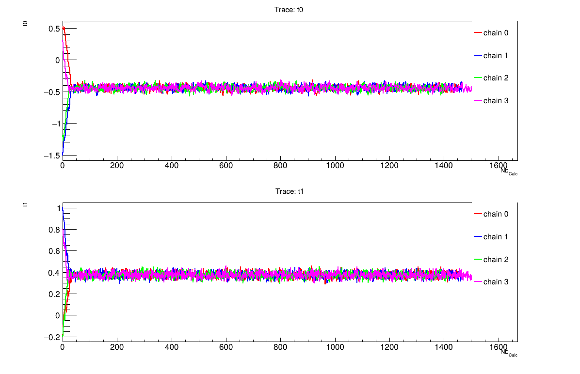
Figure 13.71 Acceptation ratio graph of the macro “calibrationMCMCLinReg.py”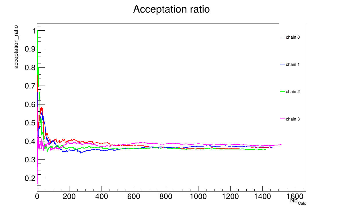
Figure 13.72 2D Trace graph of the macro “calibrationMCMCLinReg.py”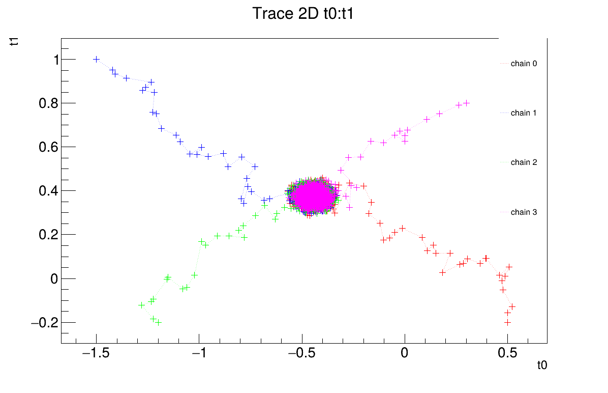
Figure 13.73 Residuals graph of the macro “calibrationMCMCLinReg.py”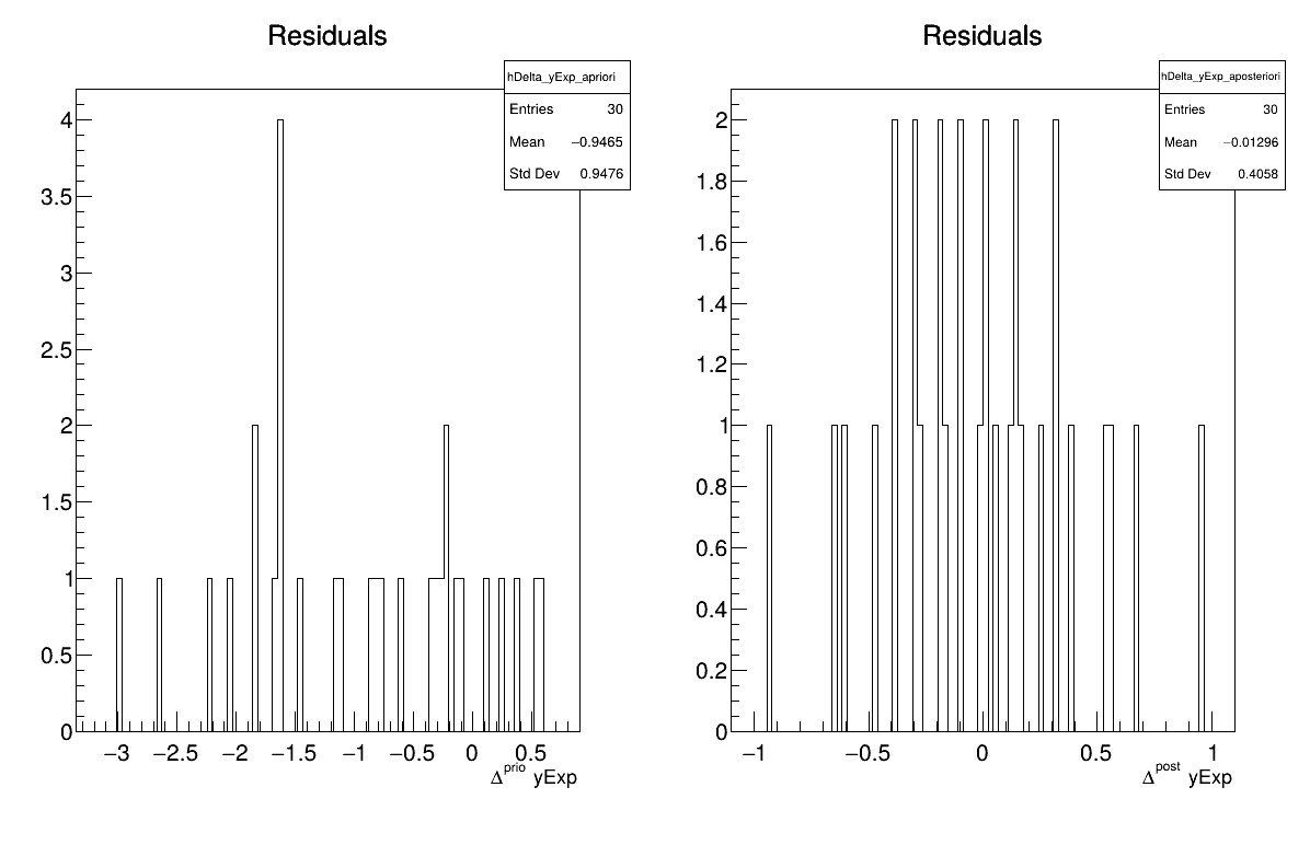
Figure 13.74 Parameter graph of the macro “calibrationMCMCLinReg.py”