

Documentation
/ Guide méthodologique
: 
| Chapter II. Basic statistical elements | ||
|---|---|---|
 |  | |
Table of Contents
This chapter introduces the various probability laws implemented in Uranie and illustrates, for each every one of them, with a few sets of parameters, the resulting shape of three of their characteristic functions. Some of the basic statistical operations are also described in a second part.
There are several already-implemented statistical laws in Uranie, that can be called marginal laws as well, used to
described the behaviour of a chosen input variable. They are usually characterised by two functions which are
intrinsically connected: the PDF (probability density function) and CDF (cumulative distribution function). One can
recap briefly the definition of these two functions for every random variable  :
:
PDF: if the random variable X has a density
 , where is a non-negative Lebesgue-integrable function, then
CDF: the function
 , given by
For some of the distributions discussed later on, the parameters provided to define them are not limiting the range
of their PDF and CDF: these distributions are said to be infinite-based ones. It is however possible to set
boundaries in order to truncate the span of their possible values. One can indeed define an lower bound
 and or an upper bound
 so that the resulting
distribution range is not infinite anymore but only in
so that the resulting
distribution range is not infinite anymore but only in  . This truncation step affects both the PDF and CDF: once the boundaries are
set, the CDF of these two values are computed to obtain
. This truncation step affects both the PDF and CDF: once the boundaries are
set, the CDF of these two values are computed to obtain  (the probability to be lower than the lower edge) and
  (the probability to be lower than the upper edge). Two new
functions, the truncated PDF
(the probability to be lower than the upper edge). Two new
functions, the truncated PDF  and the truncated CDF
  are simply defined as
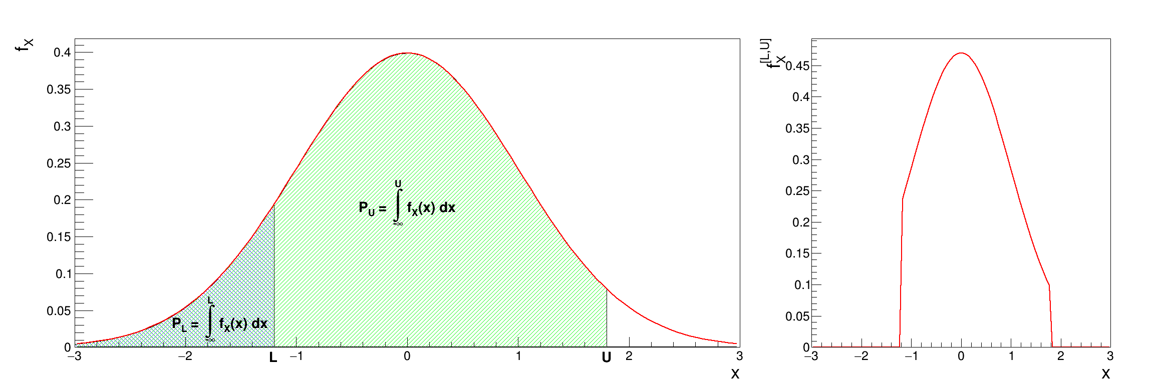
These steps to produce a truncate distribution are represented in Figure II.1 where the
original distribution is shown on the left along with the definition of (the blue shaded part) and (the green shaded part). The right part of the plot is the resulting
truncated PDF.
Figure II.1. Principle of the truncated PDF generation (right-hand side) from the orginal one (left-hand side).
 |
It is possible to combine different probability law, as a sum of weighted contributions, in order to create a new law. This approach, which is further discussed and illustrated in Section II.1.1.19, leads to a new probability density function that would look like
These distributions can be used to model the behaviour of variables, depending on chosen hypothesis, probability density function being used as a reference more oftenly by physicist, whereas statistical experts will generally use the cumulative distribution function [Appel13].
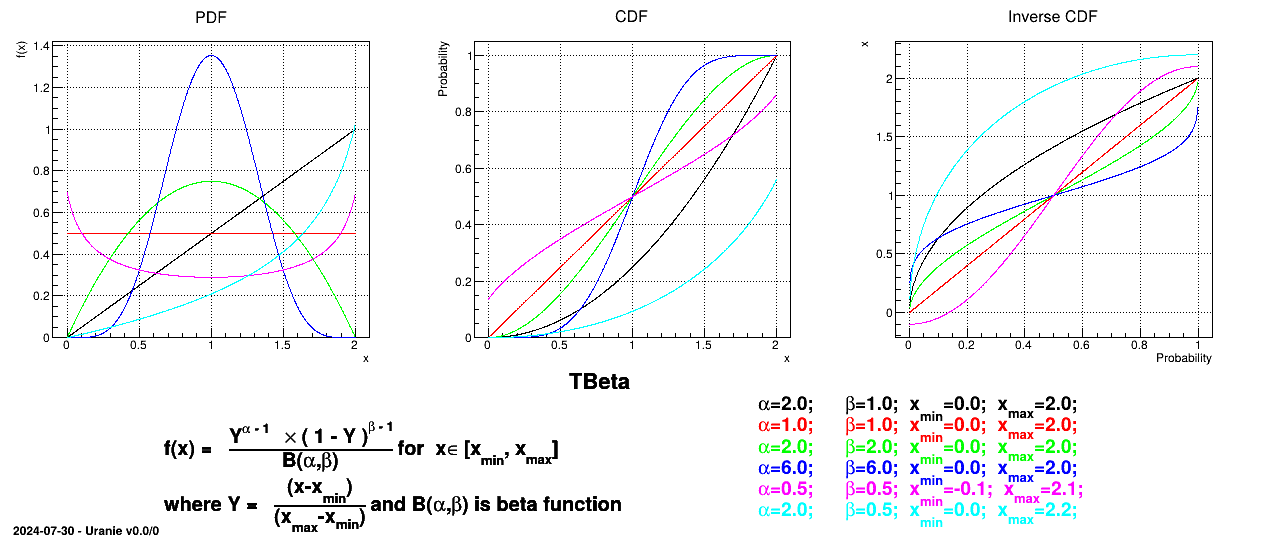
Table II.1 gathers the list of implemented statistical laws, along with the list of parameters used to define them. For every possible law, a figure is displaying the PDF, CDF and inverse CDF for different sets of parameters (the equation of the corresponding PDF is reminded as well on every figure). The inverse CDF is basically the CDF whose x and y-axis are inverted (it is convenient to keep in mind what it looks like, as it will be used to produce design-of-experiments, later-on).
Table II.1. List of Uranie classes representing the probability laws
| Law | Class Uranie | Parameter 1 | Parameter 2 | Parameter 3 | Parameter 4 |
|---|---|---|---|---|---|
| Uniform | TUniformDistribution | Min | Max | ||
| Log-Uniform | TLogUniformDistribution | Min | Max | ||
| Triangular | TTriangularDistribution | Min | Max | Mode | |
| Log-Triangular | TLogTriangularDistribution | Min | Max | Mode | |
| Normal (Gauss) | TNormalDistribution | Mean ( ) ) | Sigma ( ) ) | ||
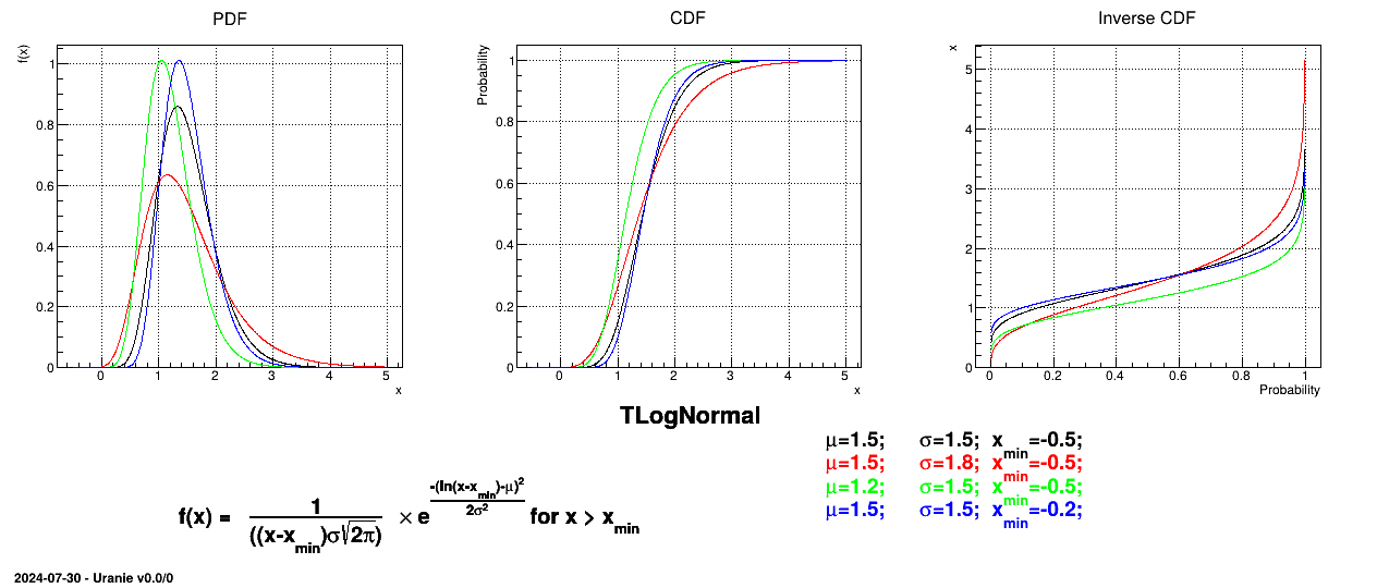
| Log-Normal | TLogNormalDistribution | Mean ( ) ) | Error factor ( ) ) | Min | |
| Trapezium | TTrapeziumDistribution | Min | Max | Low | Up |
| UniformByParts | TUniformByPartsDistribution | Min | Max | Median | |
| Exponential | TExponentialDistribution | Rate ( ) ) | Min | ||
| Cauchy | TCauchyDistribution | Scale ( ) ) | Median | ||
| GumbelMax | TGumbelMaxDistribution | Mode () | Scale ( ) )
| ||
| Weibull | TWeibullDistribution | Scale () | Shape ( ) ) | Min | |
| Beta | TBetaDistribution | alpha ( ) ) | beta () | Min | Max |
| GenPareto | TGenParetoDistribution | Location () | Scale () | Shape ( ) ) | |
| Gamma | TGammaDistribution | Shape () | Scale () | Location ( ) ) | |
| InvGamma | TInvGammaDistribution | Shape () | Scale () | Location () | |
| Student | TStudentDistribution | DoF () | |||
| GeneralizedNormal | TGeneralizedNormalDistribution | Location () | Scale () | Shape () |
//Uniform law
TUniformDistribution *pxu = new TUniformDistribution("x1", -1.0 , 1.0);
// Gaussian Law
TNormalDistribution *pxn = new TNormalDistribution("x2", -1.0 , 1.0);
// Gaussian Law
TNormalDistribution *pxn = new TNormalDistribution("x2", -1.0 , 1.0); 
Allocation of a pointer pxu to a random uniform variable x1 in interval [-1.0, 1.0]. | |
Allocation of a pointer pxn to a random normal variable x2 with mean value μ=-1.0 and standard deviation σ=1.0. |
# Uniform law
pxu = DataServer.TUniformDistribution("x1", -1.0 , 1.0)
# Gaussian Law
pxn = DataServer.TNormalDistribution("x2", -1.0 , 1.0)
Allocation of a pointer pxu to a random uniform variable x1 in interval [-1.0, 1.0]. | |
Allocation of a pointer pxn to a random normal variable x2 with mean value μ=-1.0 and standard deviation σ=1.0. |
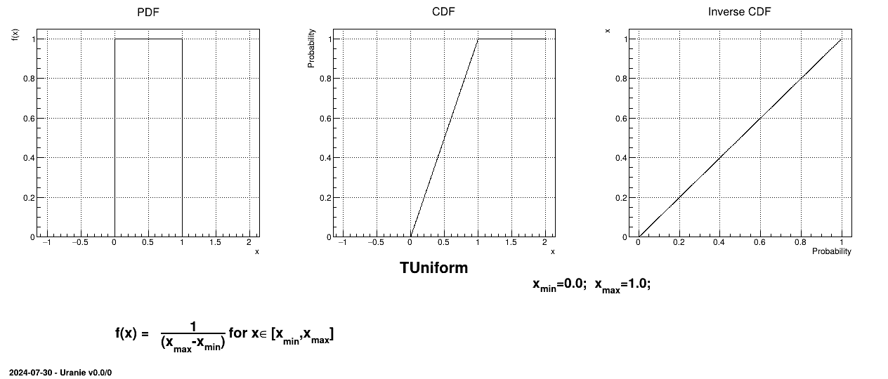
The Uniform law is defined between a minimum and a maximum, as
The property of the law
lies on the fact that all points of the interval  have the same probability. The mean value of the uniform law can
then be computed as
have the same probability. The mean value of the uniform law can
then be computed as  while its variance can be written as
 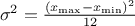 . The mode is not really defined as all points have the same probability.
Figure II.2 shows the PDF, CDF and inverse CDF generated for a given set of parameters.
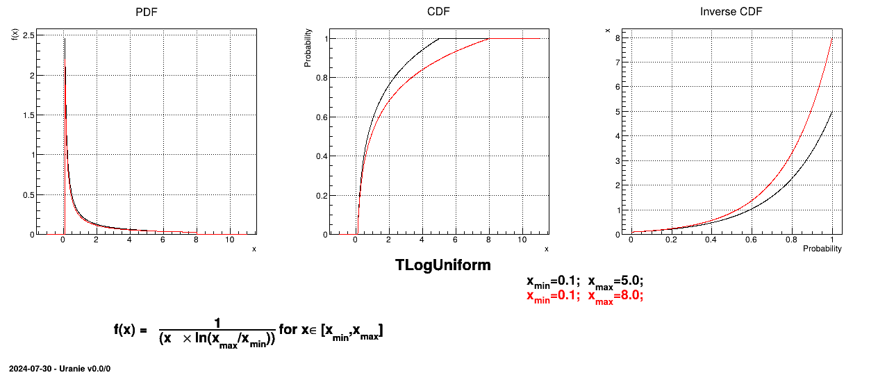
The LogUniform law is well adapted for variations of high amplitudes. If a random variable  follows a LogUniform distribution, the random variable
 follows a Uniform
distribution, so
follows a Uniform
distribution, so
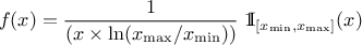
From the statistical point of
view, the mean value of the LogUniform law can then be computed as  while
its variance can be written as
while
its variance can be written as  . By definition, the mode is equal to
  .
.
Figure II.3 shows the PDF, CDF and inverse CDF generated for different sets of parameters.
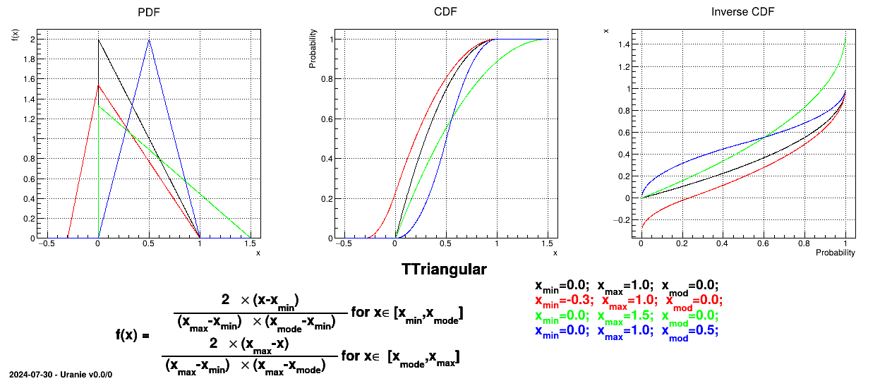
This law describes a triangle with a base between a minimum and a maximum and a highest density at a certain point
 , so
, so

The mean value of the triangular law can then be computed as  while its
variance can be written as
while its
variance can be written as  .
.
Figure II.4 shows the PDF, CDF and inverse CDF generated for different sets of parameters.
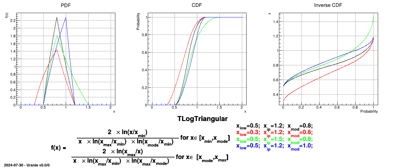
If a random variable follows a
LogTriangular distribution, the random variable follows a Triangular distribution, so

and

Figure II.5 shows the PDF, CDF and inverse CDF generated for different sets of parameters.
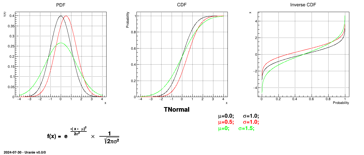
A normal law is defined with a mean (which coincide with the mode) and a standard deviation
, as
Figure II.6 shows the PDF, CDF and inverse CDF generated for different sets of parameters.
If a random variable follows a
LogNormal distribution, the random variable follows a Normal distribution (whose parameters are and ), so
In Uranie, it is parametrised by default using M, the mean of the distribution, , the Error factor that represents the ration of the
95% quantile and the median (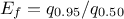 ) and the minimum
  . One can go from one parametrisation to the other following those
simple relations
. One can go from one parametrisation to the other following those
simple relations
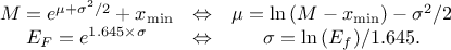
The variance of the distribution can be estimated as  while its mean is
  and its mode is
 .
.
Figure II.7 shows the PDF, CDF and inverse CDF generated for different sets of parameters.
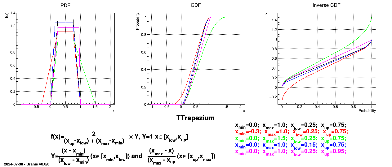
This law describes a trapezium whose large base is defined between a minimum and a maximum and its small base lies between a low and an up value, as
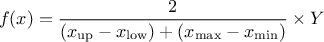
where  ,
,  and
and  .
.
For this distribution, the mean can be estimated through 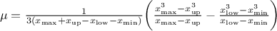 while the variance is . The mode is not properly defined as all probability are equals in
 .
.
Figure II.8 shows the PDF, CDF and inverse CDF generated for different sets of parameters.
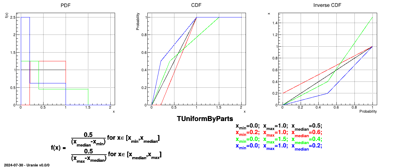
The UniformByParts law is defined between a minimum and a median and between the median and a maximum, as

For this distribution, the mean value is  while the variance is
 .
.
Figure II.9 shows the PDF, CDF and inverse CDF generated for different sets of parameters.
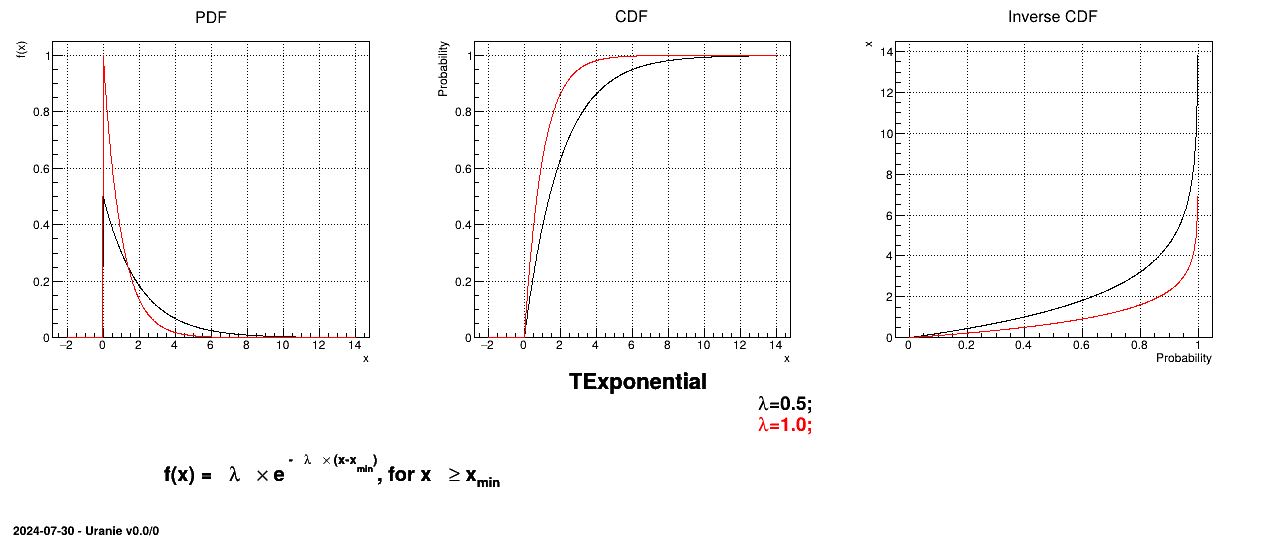
This law describes an exponential with a rate parameter and a minimum , as

The rate parameter should be positive.
The mean value of the exponential law can then be computed as  while its variance can be written as
 . The mode is the chosen minimum value.
Figure II.10 shows the PDF, CDF and inverse CDF generated for different sets of parameters.
This law describes a Cauchy-Lorentz distribution with a location parameter  and a scale parameter , as
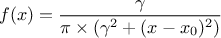
The mean and standard deviation of this distribution are not properly defined.
Figure II.11 shows the PDF, CDF and inverse CDF generated for different sets of parameters.
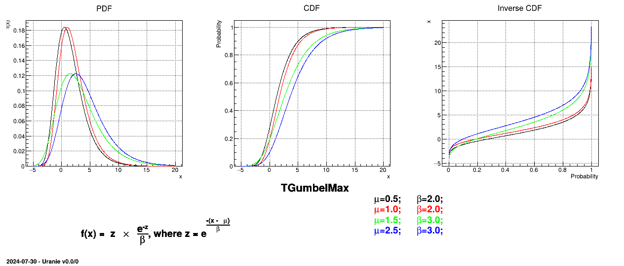
This law describes a Gumbel max distribution depending on the mode and the scale , as
The mean value of the Gumbel max law can then be computed as  , where is the Euler Mascheroni constant and its variance can be
written as
, where is the Euler Mascheroni constant and its variance can be
written as  .
.
Figure II.12 shows the PDF, CDF and inverse CDF generated for different sets of parameters.
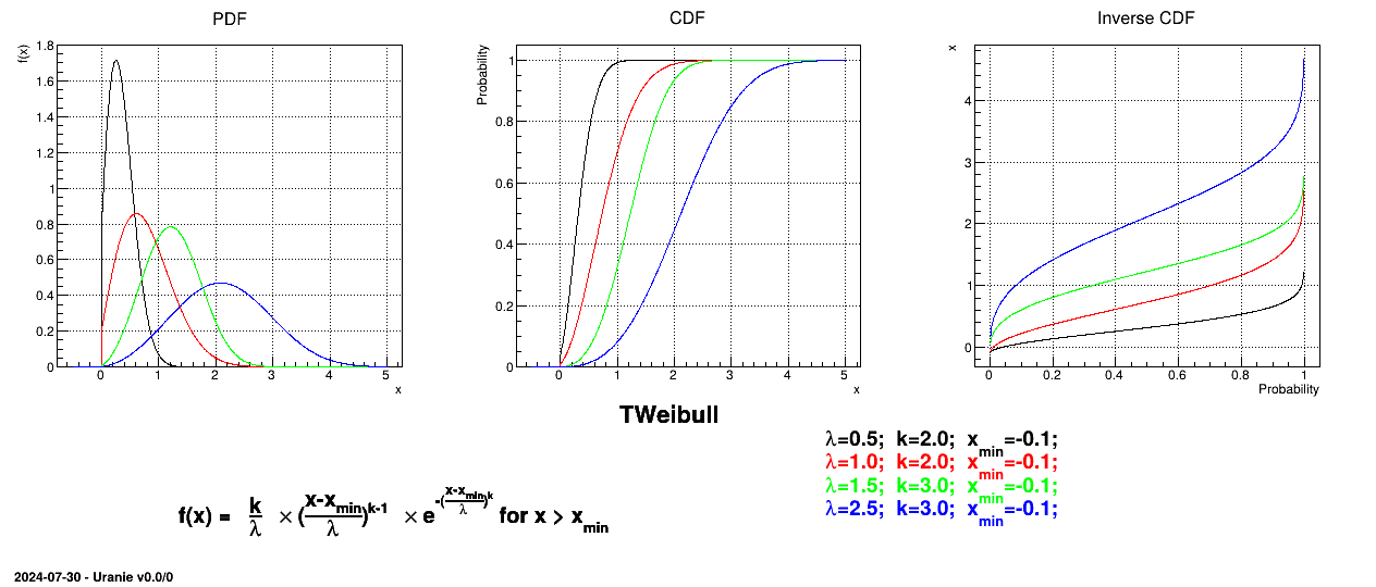
This law describes a weibull distribution depending on the location , the scale and the shape q , as
The mean value of the Weibull law can then be computed as  while its variance can be written as
 .
.
Figure II.13 shows the PDF, CDF and inverse CDF generated for different sets of parameters.
Defined between a minimum and a maximum, it depends on two parameters and , as
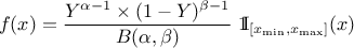
where  and
and  is the
beta function.
is the
beta function.
Figure II.14 shows the PDF, CDF and inverse CDF generated for different sets of parameters.
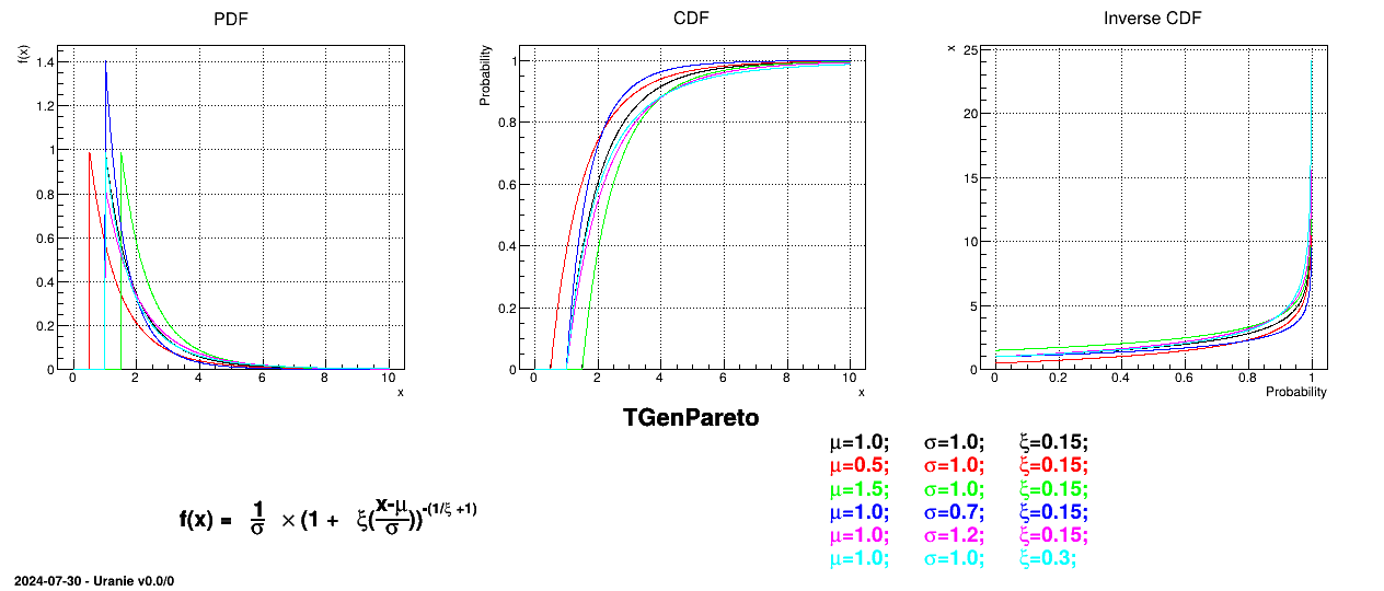
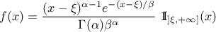
This law describes a generalised Pareto distribution depending on the location , the scale and a shape , as
In this formula, should be greater than 0. The
resulting mean for this distribution can be estimated as 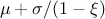 (for
(for  ) while its variance can be computed as
 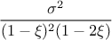 (for
(for
 ).
).
Figure II.15 shows the PDF, CDF and inverse CDF generated for different sets of parameters.
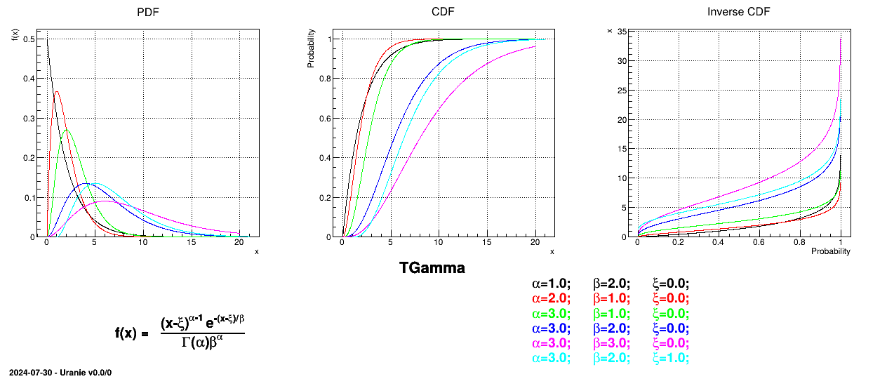
The Gamma distribution is a two-parameter family of continuous probability distributions. It depends on a shape
parameter and a scale
parameter . The function
is usually defined for greater
than 0, but the distribution can be shifted thanks to the third parameter called location () which should be positive. This
parametrisation is more common in Bayesian statistics, where the gamma distribution is used as a conjugate prior
distribution for various types of laws:
The mean value of
the Gamma law can then be computed as  while its variance can be written as
  .
.
Figure II.16 shows the PDF, CDF and inverse CDF generated for different sets of parameters.
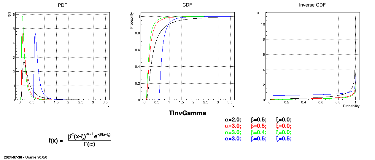
The inverse-Gamma distribution is a two-parameter family of continuous probability distributions. It depends on a shape
parameter and a scale
parameter . The function
is usually defined for greater
than 0, but the distribution can be shifted thanks to the third parameter called location () which should be positive.
The mean value of the Inverse-Gamma law can then be
computed as  (for
(for  ) while its variance can be written as
  (for
(for  ).
).
Figure II.17 shows the PDF, CDF and inverse CDF generated for different sets of parameters.
The Student law is simply defined with a single parameter: the degree-of-freedom (DoF). The probability density function is then set as
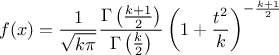
where  is the Euler's gamma function. This distribution is famous for the
t-test, a test-hypothesis developed by Fisher to check validity of the null hypothesis when the variance is
unknown and the number of degree-of-freedom is limited. Indeed, when the number of degree-of-freedom grows, the
shape of the curve looks more and more like the centered-reduced normal distribution.
The mean value of the student law is 0 as soon as
is the Euler's gamma function. This distribution is famous for the
t-test, a test-hypothesis developed by Fisher to check validity of the null hypothesis when the variance is
unknown and the number of degree-of-freedom is limited. Indeed, when the number of degree-of-freedom grows, the
shape of the curve looks more and more like the centered-reduced normal distribution.
The mean value of the student law is 0 as soon as  (and is not determined otherwise). Its variance can be written as
  as soon as
 , infinity if
 , and is not
determined otherwise.
, and is not
determined otherwise.
Figure II.18 shows the PDF, CDF and inverse CDF generated for different sets of parameters.
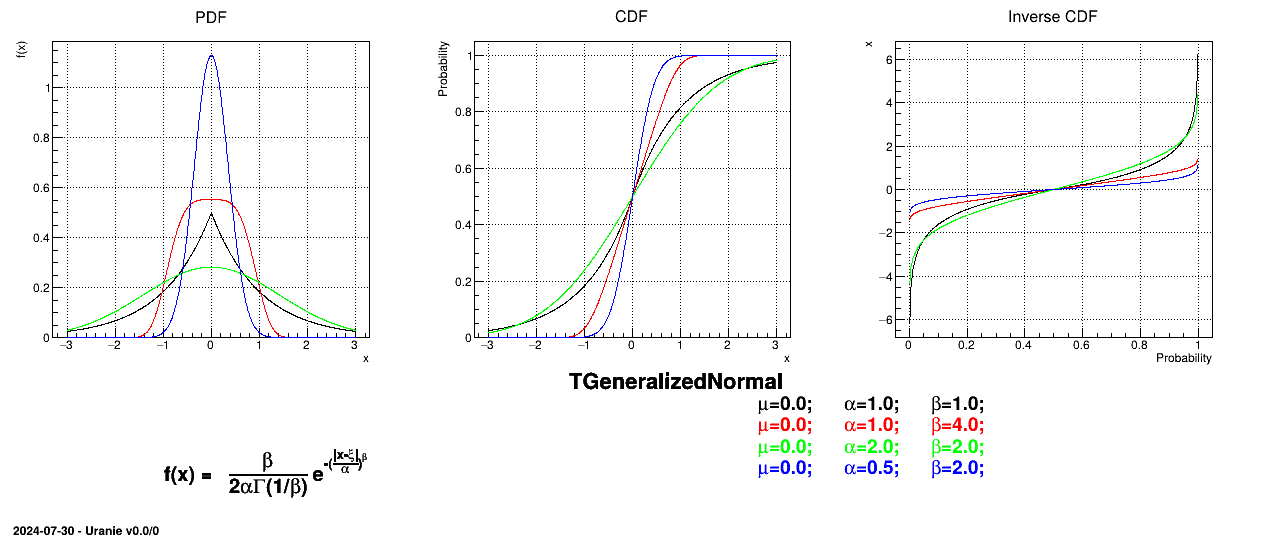
This law describes a generalized normal distribution depending on the location , the scale and the shape q , as
The mean value of the generalized normal law is  while its variance can be written as
  .
.
Figure II.19 shows the PDF, CDF and inverse CDF generated for different sets of parameters.
It is possible to imagine a new law, hereafter called composed law, by combining different
pre-existing laws in order to model a wanted behaviour. This law would be defined with  pre-existing laws whose densities are noted
 , along with their relative weights
  and the resulting density is then written as
The mean value of this newly generated law can be expressed, assuming that all pre-existing laws have a finite
and defined expectation denoted  , as
, as 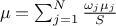 where the sum of
all weights is
where the sum of
all weights is  . As for the mean value, the variance of this newly generated
law can be expressed, assuming that all pre-existing laws have a finite and defined expectation and variance, as
done below in a very generic way.
. As for the mean value, the variance of this newly generated
law can be expressed, assuming that all pre-existing laws have a finite and defined expectation and variance, as
done below in a very generic way.
In the case of unweighted composition, this can be written as 
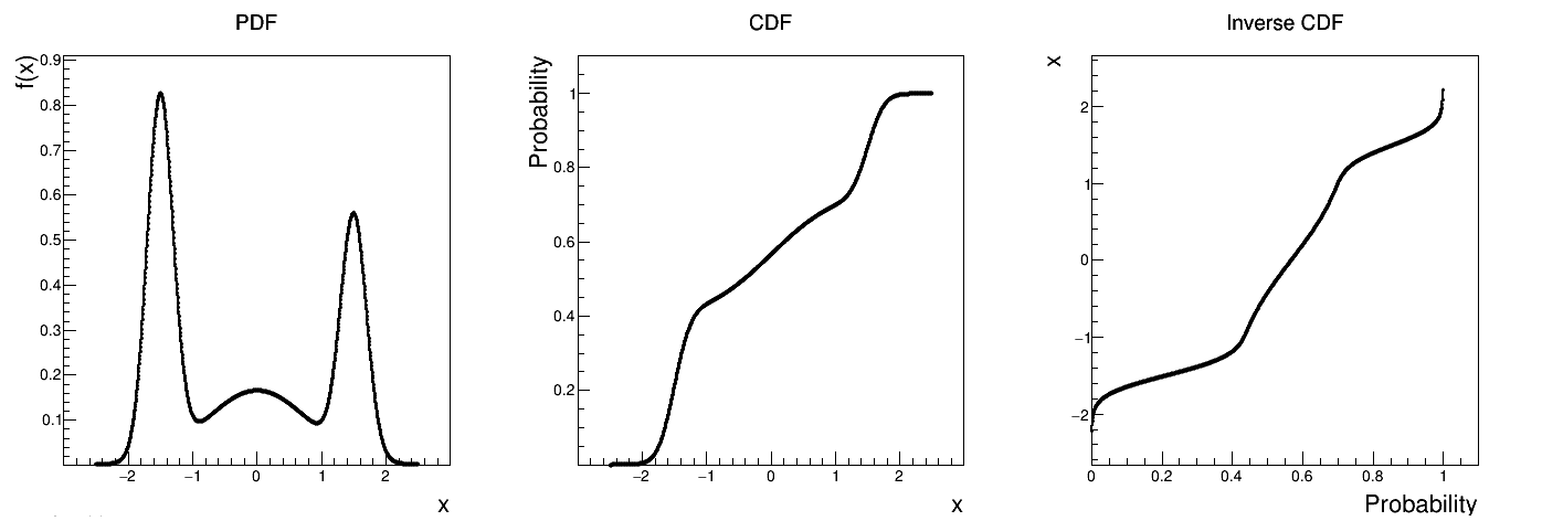
Figure II.20 shows the PDF, CDF and inverse CDF generated for different sets of parameters.
Figure II.20. Example of PDF, CDF and inverse CDF for a composed distribution made out of three normal distributions with respective weights.
 |
| | | |
| Chapter I. Glossary |  | II.2. Statistical treatments and operations |