

Documentation
/ Methodological guide
: 
| II.2. Statistical treatments and operations | ||
|---|---|---|
 | Chapter II. Basic statistical elements |  |
There are many different kinds of operations that can be applied on an existing set of data
(disregarding their origin, i.e. whether they come from experiments, simulations...). They are all
listed below and the main ones are described in more details in the following subsections. For the sake of simplicity,
the input variable is called  leading to an output variable called
  . The dataset contains
  points and
  is be
an iterator that goes from 0 to
is be
an iterator that goes from 0 to  . In few words, here what's easily calculable with Uranie:
The normalisation of variable, in Section II.2.1
The ranking of variable, in Section II.2.2
The elementary statistic computation, in Section II.2.3
The quantile estimation, in Section II.2.4
The correlation matrix determination, in Section II.2.5
The normalisation function can be called to create new variables, for every requested normalisation, whose range and dispersion depend on the chosen normalisation method. Up to now, there are four different ways to perform this normalisation:
centered-reducted: the new variable values are computed as

centered: the new variable values are computed as

reduced to
 :
the new variable values are computed as
:
the new variable values are computed as 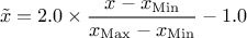
reduced to
 : the
new variable values are computed as
: the
new variable values are computed as 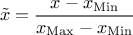
The ranking of variable is used in many methods that are focusing more on monotony than on linearity (this is
discussed throughout this documentation when coping with regression, correlation matrix, c.f. for instance Section V.1.1.2). The way this is done in Uranie is the following: for every variable considered,
a
new variable is created, whose name is constructed as the name of the considered variable with the prefix "Rk_". The
ranking consists in assigning to each
variable entry an integer, that goes from 1 to the number of patterns, following an order relation (in Uranie it is
chosen so that 1 is the smallest value and is the largest one).
When considering an existing set of
points, it exists a method to determine the four simplest statistical notions: the minimum, maximum, average
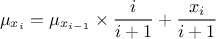
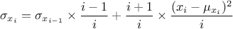
and standard deviation. The minimum and maximum are trivially estimated by running over all
the possible values. The average and standard deviation are estimated on the fly, using the following recursive
formulae (where  represents the value of
  using all data points up to for
 ):
):


There are several ways of estimating the quantiles implemented in Uranie. This part describes the most commonly used and starts with a definition of quantile.
A quantile  , as
discussed in the following parts, for p a probability going from 0 to 1, is the lowest value of the random variable
, as
discussed in the following parts, for p a probability going from 0 to 1, is the lowest value of the random variable
 leading to
  . This definition
holds equally if one is dealing with a given probability distribution (leading to a theoretical quantile), or a
sample, drawn from a known probability distribution or not (leading to an empirical quantile). In the latter case,
the sample is split into two sub-samples: one containing
. This definition
holds equally if one is dealing with a given probability distribution (leading to a theoretical quantile), or a
sample, drawn from a known probability distribution or not (leading to an empirical quantile). In the latter case,
the sample is split into two sub-samples: one containing  points, the other one containing
  points.
For a given probability  , the
corresponding quantile
, the
corresponding quantile  is given
by:
is given
by:
where
 is the k-Th smallest value of the variable set-of-value (whose size is
). The way the index
is the k-Th smallest value of the variable set-of-value (whose size is
). The way the index  is computed depends on how conservative one wants to be,
but also on the case under consideration. For discontinuous cases, one can choose amongst the following list:
is computed depends on how conservative one wants to be,
but also on the case under consideration. For discontinuous cases, one can choose amongst the following list:


 , approximately median unbiased.
 , approximately unbiased if is normally distributed.
The Wilks quantile computation is an empirical estimation, based on order statistic which allows to get an
estimation on the requested quantile, with a given confidence level  , independently of the nature of the law, and most of the time,
requesting less estimations than a classical estimation. Going back to the empirical way discussed in Section II.2.4.1: it consists, for a 95% quantile, in running 100 computations, ordering the
obtained values and taking the one at either the 95-Th or 96-Th position (see the discussion on how to choose k in
Section II.2.4.1). This can be repeated several times and will result in a
distribution of all the obtained quantile values peaking at the theoretical value, with a standard deviation
depending on the number of computations made. As it peaks on the theoretical value, 50% of the estimation are
larger than the theoretical value while the other 50% are smaller (see Figure II.21 for illustration purpose).
, independently of the nature of the law, and most of the time,
requesting less estimations than a classical estimation. Going back to the empirical way discussed in Section II.2.4.1: it consists, for a 95% quantile, in running 100 computations, ordering the
obtained values and taking the one at either the 95-Th or 96-Th position (see the discussion on how to choose k in
Section II.2.4.1). This can be repeated several times and will result in a
distribution of all the obtained quantile values peaking at the theoretical value, with a standard deviation
depending on the number of computations made. As it peaks on the theoretical value, 50% of the estimation are
larger than the theoretical value while the other 50% are smaller (see Figure II.21 for illustration purpose).
Wilks computation on the other hand request not only a probability value but also a confidence level. The quantile
 represents the
quantile given the
probability but this time, the
value is provided with a % confidence level, meaning that % of the obtain value is larger than the theoretical quantile. This is a way to be
conservative and to be able to quantify how conservative one wants to be. To do this, the size of the sample must
follow a necessary condition:
represents the
quantile given the
probability but this time, the
value is provided with a % confidence level, meaning that % of the obtain value is larger than the theoretical quantile. This is a way to be
conservative and to be able to quantify how conservative one wants to be. To do this, the size of the sample must
follow a necessary condition:
This is the smallest sample size to get an estimation, and, in most cases, the accuracy reached (for a given sample size) is better than the one achieved with the simpler solution provided above. It is also possible to increase the sample size to get a better description of the quantile estimation.
Figure II.21. Illustration of the results of 100000 quantile determinations, applied to a reduced centered gaussian distribution, comparing the usual and Wilks methods. The number of points in the reduced centered gaussian distribution is varied, as well as the confidence level.
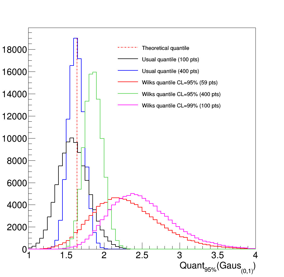 |
Figure II.21 shows a simple case: the estimation of the value of the 95% quantile of a centered-reduced normal distribution. The theoretical value (red dashed line) is compared to the results of 100000 empirical estimation, following the simple recipe (black and blue curves) or the Wilks method (red, green and magenta curves). Several conclusions can be drawn:
The simpler quantile estimation average is slightly biased with respect to the theoretical value. This is due to the choice of k, discussed in Section II.2.4.1 which can lead to under or over estimation of the quantile value. The bias becomes smaller with the increasing sample size.
The standard deviation of the distributions (whatever method is considered) is becoming smaller with the increasing sample size.
When using the Wilks method, the fraction of event below the theoretical value is becoming smaller with the increasing confidence level.
The computation of the correlation matrix can be done either on the values (leading to the Pearson coefficients) or on the ranks (leading to the Spearmann coefficients).
Correlation matrices are computed in a 3 steps procedure detailed below:
An overall
 matrix is
created and filled, every line being a new entry while every column is a variable
matrix is
created and filled, every line being a new entry while every column is a variable
This matrix is centred and reduced: for every variable under consideration
 is subtracted and the results is divided by
 .
.
The resulting correlation matrix is obtained from the product

| |  | |
| Chapter II. Basic statistical elements |  | II.3. Combining these aspects: performing PCA |