

Documentation
/ Guide méthodologique
: 
| II.3. Combining these aspects: performing PCA | ||
|---|---|---|
 | Chapter II. Basic statistical elements |  |
This part is introducing an example of analysis that combines all the aspects discussed up to now: handling data, perform a statistical treatment and visualise the results. This analysis is called PCA for Principal Component Analysis and is often used to
gather event in a sample that seem to have a common behaviour;
reduce the dimension of the problem under study.
There is a very large number of articles, even books, discussing the theoretical aspects of principal component analysis (for instance one can have a look at [jolliffe2011principal]).
The principle of this kind of analysis is to analyse a provided ensemble, called hereafter  , whose size is
  , and which can be written as
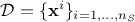
where  is the i-Th input vector, written as
 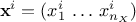 where
where  is the number of
quantitative variable. It is basically a set of realisation of random variables whose properties are completely unknown.
is the number of
quantitative variable. It is basically a set of realisation of random variables whose properties are completely unknown.
The aim is then to summarise (project/reduce) this sample into a smaller dimension space  (with
(with  ) these factors being chosen in order to maximise the inertia and being orthogonal one to
another[1]. By doing so, the goal is to be able to reduce the dimension of our problem
while loosing as few information as possible.
) these factors being chosen in order to maximise the inertia and being orthogonal one to
another[1]. By doing so, the goal is to be able to reduce the dimension of our problem
while loosing as few information as possible.
If one calls  the original sample whose dimension is
  , the idea behind PCA is to find the projection matrix
  , whose dimension is
  , that would re-express the data
optimally as a new sample, called hereafter
, that would re-express the data
optimally as a new sample, called hereafter  , with the same dimension . The rows of are forming a new basis to represent the column of and this new basis will later
become our principal component directions.
, with the same dimension . The rows of are forming a new basis to represent the column of and this new basis will later
become our principal component directions.
Now recalling the aim of PCA, the way to determine this projection matrix is crucial and should be designed as to
find out the best linear combinations between variables so that the minimum number of rows (principal components) of
are considered useful to carry on as much inertia as possible;
rank the principal component so that, if not satisfy with the new representation, it would be simple to add an extra principal component to improve it.
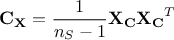
This can be done by investigating the covariance matrix  of that, by definition, describes the linear combination between variables and
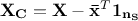
that could be computed from the centered matrix sample
of that, by definition, describes the linear combination between variables and
that could be computed from the centered matrix sample  [2]as
[2]as
If one consider the resulting covariance matrix  , the aim is to maximise the signal measured by variance (diagonal entries
that represents the variance of the principal components) while minimising the covariance between them. As the
lowest covariance value reachable is 0, if the desired covariance matrix would append to be diagonal, this would mean
our objectives are achieved. From the very definition of the covariance matrix, one could see that
, the aim is to maximise the signal measured by variance (diagonal entries
that represents the variance of the principal components) while minimising the covariance between them. As the
lowest covariance value reachable is 0, if the desired covariance matrix would append to be diagonal, this would mean
our objectives are achieved. From the very definition of the covariance matrix, one could see that

As is
symmetric, it is orthogonal diagonalisable, and can be written  . In this equation,
 is an
orthonormal matrix whose columns are the orthonormal eigenvectors of , and
is an
orthonormal matrix whose columns are the orthonormal eigenvectors of , and  is a diagonal matrix which has the eigenvalues of
. Given
this, if we choose
is a diagonal matrix which has the eigenvalues of
. Given
this, if we choose  , this leads to

At this level, there is no
unicity of the
matrix as one can have many permutations of the eigenvalues along the diagonal, as long as one changes
accordingly.
Finally, an interesting link can be drawn between this protocol and a very classical method of linear algebra, already mentioned in other places of this document, called the Singular Value Decomposition (SVD[3]) leading to

In
this context  and
and  are unitary
matrices (also known as respectively the left singular vectors and right singular
vectors of
are unitary
matrices (also known as respectively the left singular vectors and right singular
vectors of  ) while
  is a diagonal matrix storing the singular values of in decreasing
order. The last step is then to state the linear algebra theorem which says that the non-zero singular values of
are
the square roots of the nonzero eigenvalues of
is a diagonal matrix storing the singular values of in decreasing
order. The last step is then to state the linear algebra theorem which says that the non-zero singular values of
are
the square roots of the nonzero eigenvalues of  and
and  (the corresponding eigenvectors being the
columns of respectively
(the corresponding eigenvectors being the
columns of respectively  and
and  ).
).
Gathering all this, one can see that by doing the SVD on the centered original sample matrix, the resulting
projection matrix can be identified as  and the resulting covariance matrix will be proportional to
 . The final interesting property is coming from the SVD itself: as gathers the
eigenvalues in decreasing order, it assures the unicity of the transformation and give access to the principal
component in a hierarchical way.
. The final interesting property is coming from the SVD itself: as gathers the
eigenvalues in decreasing order, it assures the unicity of the transformation and give access to the principal
component in a hierarchical way.
From what has been discussed previously it can appear very appealing, but there are few drawbacks or at least limitations that can be raised:
This method is very sensitive to extreme points: correlation coefficient can be perturbed by them.
In the case of non-linear phenomenon, the very basic concept of PCA collapses. Imagine a simple circle-shaped set of points, there are no correlation between the two variables, so no smaller space can be found using linear combinations.
Even if the PCA is working smoothly, one has to be able to find an interpretation of the resulting linear combinations that have been defined to create the principle component. Moreover, it might not be possible to move along on more refined analysis, such as sensitivity analysis for instance.
[1] As a reminder, the dispersion of a quantitative variable is usually represented with its variance (or standard deviation), the inertia criteria is, for multi-dimension problems, the sum of all the variable's variance.
[2] The centered matrix is defined as
 where
where  is the vector of mean value for every variable and
  is a vector of 1 whose
dimension is .
is a vector of 1 whose
dimension is .
[3] SVD is applied to matrix whose number of rows should be greater than its number of columns.
| |  | |
| II.2. Statistical treatments and operations |  | Chapter III. The Sampler module |