

Documentation
/ Guide méthodologique
: 
| III.2. The Stochastic methods | ||
|---|---|---|
 | Chapter III. The Sampler module |  |
In these methods the knowledge (or mis-knowledge) of the model is encoded in the choice of probability
law used to describe the inputs  , for
, for  . These laws are usually defined by:
a range that describes the possible values of
the nature of the law, which has to be taken in the list of pre-defined laws already presented in Section II.1.1
A choice has frequently to be made between two implemented methods of drawing:
- SRS (Simple Random Sampling):
This method consists in independently generating the samples for each parameter following its own probability density function. The obtained parameter variance is rather high, meaning that the precision of the estimation is poor leading to a need for many repetitions in order to reach a satisfactory precision. An example of this sampling when having two independent random variables (uniform and normal one) is shown in Figure III.3-left. In order to get this drawing, the variable are normalised from 0 to 1 and a random drawing is performed in this range. The obtained value is computed calling the inverse CDF function corresponding to the law under study (that one can see from Figure II.2 until Figure II.18).
- LHS (Latin Hypercube Sampling):
this method [McKay2000] consists in partitioning the interval of each parameter so as to obtain segments of equal probabilities, and afterwards in selecting, for each segment, a value representing this segment. An example of this sampling when having two independent random variables (uniform and normal one) is shown in Figure III.3-right. In order to get this drawing, the variable are normalised from 0 to 1 and this range is split into the requested number of points for the design-of-experiments. Thanks to this, a grid is prepared, assuring equi-probability in every sub-space. Finally, a random drawing is performed in every sub-range. The obtained value is computed calling the inverse CDF function corresponding to the law under study (that one can see from Figure II.2 until Figure II.18).
The first method is fine when the computation time of a simulation is "satisfactory". As a matter of fact, it has the
advantage of being easy to implement and to explain; and it produces estimators with good properties not only for the
mean value but also for the variance. Naturally, it is necessary to be careful in the sense to be given to the term
"satisfactory". If the objective is to obtain quantiles for extreme probability values  (i.e. = 0.99999 for instance), even for a very
low computation time, the size of the sample would be too large for this method to be used. When a computation time
becomes important, the LHS sampling method is preferable to get robust results even with small-size samples
(i.e.
(i.e. = 0.99999 for instance), even for a very
low computation time, the size of the sample would be too large for this method to be used. When a computation time
becomes important, the LHS sampling method is preferable to get robust results even with small-size samples
(i.e.  = 50 to 200) [Helton02]. On the other hand, it is rather trivial to double the
size of an existing SRS sampling, as no extra caution has to be taken apart from the random seed.
= 50 to 200) [Helton02]. On the other hand, it is rather trivial to double the
size of an existing SRS sampling, as no extra caution has to be taken apart from the random seed.
In Figure III.2, we present two samples of size = 8 coming from these two sampling methods for two
random variables  according to
a gaussian law, and
according to
a gaussian law, and  a uniform
law. To make the comparison easier, we have represented on both figures the partition grid of equiprobable segments
of the LHS method, keeping in mind that it is not used by the SRS method. These figures clearly show that for LHS
method each variable is represented on the whole domain of variation, which is not the case for the SRS method. This
latter gives samples that are concentrated around the mean vector; the extremes of distribution being, by definition,
rare.
a uniform
law. To make the comparison easier, we have represented on both figures the partition grid of equiprobable segments
of the LHS method, keeping in mind that it is not used by the SRS method. These figures clearly show that for LHS
method each variable is represented on the whole domain of variation, which is not the case for the SRS method. This
latter gives samples that are concentrated around the mean vector; the extremes of distribution being, by definition,
rare.
Concerning the LHS method (right figure), once a point has been chosen in a segment of the first variable , no other point of this segment will be picked
up later, which is hinted by the vertical red bar. It is the same thing for all other variables, and this process is
repeated until the
points are obtained. This elementary principle will ensure that the domain of variation of each variable is totally
covered in a homogeneous way. On the other hand, it is absolutely not possible to remove or add points to a LHS
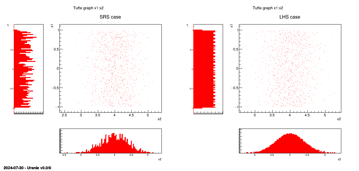
sampling without having to regenerate it completely. A more realistic picture is draw in Figure III.3 with the same laws, both for SRS on the left and LHS on the right which clearly shows the
difference between both methods when considering one-dimensional distribution.
Figure III.2. Comparison of the two sampling methods SRS (left) and LHS (right) with samples of size 8.
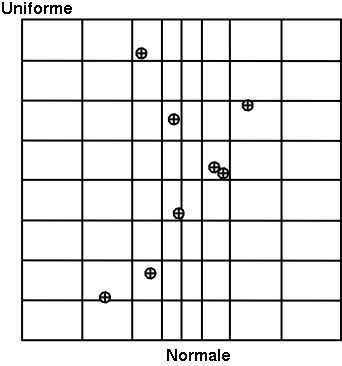
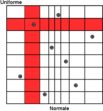
Figure III.3. Comparison of deterministic design-of-experiments obtained using either SRS (left) or LHS (right) algorithm, when having two independent random variables (uniform and normal one)
 |
There are two different sub-categories of LHS design-of-experiments discussed here and whose goal might slightly differs from the main LHS design discussed above:
the maximin LHS: this category is the result of an optimisation whose purpose is to maximise the minimal distance between any sets of two locations. This is discussed later-on in Section III.2.3.
the constrained LHS: this category is defined by the fact that someone wants to have a design-of-experiments fulfilling all properties of a Latin Hypercube Design but adding one or more constraints on the input space definition (generally inducing correlation between varibles). This is also further discussed in Section III.2.4.
Once the nature of the law is chosen, along with a variation range, for all inputs , the correlation between these variables has to be taken
into account. It is doable by defining a
correlation coefficient but the way it is treated from one sampler to the other is tricky and is further discussed in
the next section.
This section is introducing the way Uranie classes are introducing correlation between random variables when considering either the Pearson of Spearman correlation coefficients. The idea is to better explain the expected behaviour while remaining at this level of correlation description (not going deep into the copula notion).
Let start by discussing the definition of a correlation matrix that connect (or not) a variable with the
others. For a given problem with  variables, the covariance between two variables (denoted
  ) and their linear correlation
(denoted
) and their linear correlation
(denoted  )
can be estimated as
)
can be estimated as

In the equation above  and
and
 are respectively the
mean and standard deviation of the random variable under consideration. The coefficients that should be provided by
the user are the correlation one, called the Pearson ones (as they've been estimated using values of the random
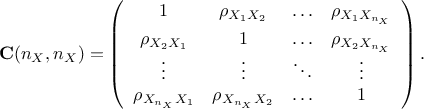
variables, but this is further discussed at the end of this section and also in Section V.1.1). The idea is to gather all these coefficients in matrix, called hereafter the correlation
matrix, that can be written as
are respectively the
mean and standard deviation of the random variable under consideration. The coefficients that should be provided by
the user are the correlation one, called the Pearson ones (as they've been estimated using values of the random
variables, but this is further discussed at the end of this section and also in Section V.1.1). The idea is to gather all these coefficients in matrix, called hereafter the correlation
matrix, that can be written as
Depending on the reference, one can discuss either the correlation matrix ( ) or the covariance matrix (
 ). Going from one to the other
is trivial if one defines
). Going from one to the other
is trivial if one defines  the diagonal matrix of dimension whose coefficients are the standard deviation of the random variables, then

Let's assume we have a random drawing  , where every column is the drawing of a given random variable of size
 . On can then compute the
following matrix
. On can then compute the
following matrix 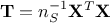 which is the correlation matrix (respectively covariance matrix) of our
sample, if the columns have been centered and reduced (respectively only centered). If were to be infinite, we would be able to state
that the resulting empirical correlation of the drawn marginal would asymptotically be the identity matrix of
dimension , noted
which is the correlation matrix (respectively covariance matrix) of our
sample, if the columns have been centered and reduced (respectively only centered). If were to be infinite, we would be able to state
that the resulting empirical correlation of the drawn marginal would asymptotically be the identity matrix of
dimension , noted
 .
.
The next step is then to correlate the variable so that  is not the identity anymore but the target correlation matrix
 . Knowing that when one multiplies a matrix of random samples by a matrix
  to get
  , the
resulting variance is estimated as [MatCook]
, the
resulting variance is estimated as [MatCook]
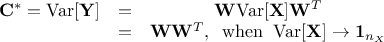
This leads to the fact that the transformation matrix that
provides such a correlation matrix in the end should satisfy the last line of previous equation which is the
definition of the Cholesky decomposition of an hermitian positive-definite matrix (W being a lower triangular
matrix)

These steps are the one used to correlate the variables in
both in the TBasicSampling and TGaussianSampling classes. Let's call
this method the simple decomposition.
The implementation done in the TSampling class, is far more tricky to understand and the aim
is not to explain the full concept of the method, called the Iman and Conover method
[Iman82]. The rest of this paragraph will just provide insight on what's done specifically to
deal with the correlation part which is different from what's been explained up to now. The main difference is
coming from the underlying hypothesis, written in the second line of Equation III.2: in a perfect
world, for a given random drawing of uncorrelated variables the correlation matrix should satisfy the relation
 . This is obviously not the case[4], so one of the proposal to
overcome this is to perform a second Cholesky decomposition, on the drawn sample correlation matrix, to get the
following decomposition:
. This is obviously not the case[4], so one of the proposal to
overcome this is to perform a second Cholesky decomposition, on the drawn sample correlation matrix, to get the
following decomposition:  . As
. As  is lower triangular, it is rather trivial to invert, we can then consider to
transform the generated sample using this relation:
is lower triangular, it is rather trivial to invert, we can then consider to
transform the generated sample using this relation: ![]() . If one consider that these multiplication does not change the fact that columns are centered and
reduced, then one can write the following equations
. If one consider that these multiplication does not change the fact that columns are centered and
reduced, then one can write the following equations
Thanks to this procedure (and many more technicalities such as, for instance, working with Spearman coefficient to be able to handle correlation with stratified samples) the resulting correlation matrix is designed to be as close as possible to the target one.
The final part of this discussion is a limitation of both methods: relying on Cholesky decomposition to decompose the
target correlation matrix. If one considers the case where  is a singular matrix, then two important points can be raised:
this case means that one or more variables can be completely defined thanks to the others. The number of properly defined variable can then be estimated by the rank of the correlation matrix. This situation can occur, as in some complicated problem variables can be highly-intricated leading to this kind of situation.
with this kind of correlation matrix, the Cholesky decomposition is not doable anymore so both methods are meant to stop brutally.
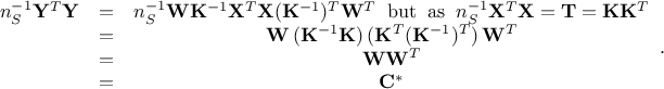
In order to overcome this situation we propose to use a workaround based on the Singular Value Decomposition
(SVD) which leads to, knowing that is real symmetric, 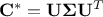 . This writing emphasise the connection between SVD and eigenvalue decomposition (for a more
general form and SVD, see for instance Equation II.2). In this context,
. This writing emphasise the connection between SVD and eigenvalue decomposition (for a more
general form and SVD, see for instance Equation II.2). In this context,  is an unitary
matrices while
is an unitary
matrices while  is a diagonal matrix storing the singular values of
in
decreasing order. In our case, where the correlation is singular, it means that one or more of the singular values
are very close or equal to 0. By rewriting our decomposition as below
is a diagonal matrix storing the singular values of
in
decreasing order. In our case, where the correlation is singular, it means that one or more of the singular values
are very close or equal to 0. By rewriting our decomposition as below

one can redefine the matrix  and get the usual formula discussed above (see Equation III.3). This decomposition can then be used instead of the Cholesky decomposition in both
method (as it is either for the simple form or along with another Cholesky to decompose the correlation matrix of
the drawn sample, in our modified Iman and Conover algorithm).
and get the usual formula discussed above (see Equation III.3). This decomposition can then be used instead of the Cholesky decomposition in both
method (as it is either for the simple form or along with another Cholesky to decompose the correlation matrix of
the drawn sample, in our modified Iman and Conover algorithm).
The usage of an SVD instead of a Cholesky decomposition for the target correlation matrix relies on the underlying
hypothesis that the left singular vectors ( ) can be used instead of the right singular
vectors () in the general SVD formula shown for instance in Equation II.2. This holds even
for the singular case, as the only differences seen between both singular vector basis arise for the singular values
close to zero. Since in this method we are always using the singular vector matrix weighted by the square roots of
the singular values, these differences are vanishing by construction.
) can be used instead of the right singular
vectors () in the general SVD formula shown for instance in Equation II.2. This holds even
for the singular case, as the only differences seen between both singular vector basis arise for the singular values
close to zero. Since in this method we are always using the singular vector matrix weighted by the square roots of
the singular values, these differences are vanishing by construction.
Considering the definition of a LHS sampling, introduced in Section III.2.1, it is clear that permutating a coordinate of two different points, will create a new sampling. If one looks at the x-coordinate (corresponding to a normal distribution) in Figure III.2, one could put the point in the second equi-probable range, in the sixth one, and move the point which was in the sixth equi-probable range into the second one, without changing the y-coordinate. The results of this permutation is a new sampling with the interesting property of remaining a LHS sampling. A follow-up question can then be: what is the difference between these two samplings, and would there be any reason to try many permutations ?
This is a very brief introduction to a dedicated field of research: the optimisation of a design-of-experiments with respect to the
goals of the ongoing analysis. In Uranie, a new kind of LHS sampling has been recently introduced, called maximin
LHS, whose purpose is to maximise the minimal distance between two points. The distance under consideration is the
mindist criterion: let 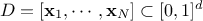 be
a design-of-experiments with
be
a design-of-experiments with  points. The mindist criterion is written as:
where  is the euclidian norm. The designs which maximise the
mindist criterion are referred to as maximin LHS, but generally speaking, a design with a large value of the
mindist criterion is referred to as maximin LHS as well. It has been observed that the best designs in terms of
maximising (Equation III.4) can be constructed by minimising its
is the euclidian norm. The designs which maximise the
mindist criterion are referred to as maximin LHS, but generally speaking, a design with a large value of the
mindist criterion is referred to as maximin LHS as well. It has been observed that the best designs in terms of
maximising (Equation III.4) can be constructed by minimising its  regularisation instead. It is written as
Figure III.4 shows, on the left, an example of a LHS when considering a problem with two uniform distributions between 0 and 1 but also, on the right, its transformation through the maximin optimisation. The mindist criterion is displayed on top for comparison purpose.
Figure III.4. Transformation of a classical LHS (left) to its corresponding maximin LHS (right) when considering a problem with two uniform distributions between 0 and 1.
From a theoretical perspective, using a maximin LHS to build a Gaussian process (GP) emulator can reduce the predictive variance when the distribution of the GP is exactly known. However, it is not often the case in real applications where both the variance and the range parameters of the GP are actually estimated from a set of learning simulations run over the maximin LHS. Unfortunately, the locations of maximin LHS are far from each other, which is not a good feature to estimate these parameters with precision. That is why maximin LHS should be used with care. Relevant discussions dealing with this issue can be found in [Pronz12].
The Simulated Annealing (SA) algorithm is a probabilistic metaheuristic which can solve a global optimisation problem. It is here applied to the construction of maximin Latin Hypercube Designs (maximin LHS). The SA algorithm consists in exploring the space of LHS through elementary random perturbations of both rows and columns in order to converge to maximin ones. We have implemented in Uranie the algorithm of Morris and Mitchell [Morris95,Dam13], which is driven by the following parameters
 is the
initial temperature
is the
initial temperature- the decreasing of the temperature is controlled by

- the number of iterations in the outer loop

- the number of iterations in the inner loop

It is important to keep in mind that the performances of the simulated annealing method can strongly depend on
and thus changing
parametrisation can lead to disappointing results. Below, in Table III.1, we
provide some parametrisation examples working well with respect both to the number of the input variables
 and the size of the requested
design .
and the size of the requested
design .
Table III.1. Proposed list of parameters value for simulated annealing algorithm, depending on the number of points
requested () and the number of
inputs under consideration ()
|  |  |  | |||
|---|---|---|---|---|---|---|
| 2,3,4 | | 0.99 | | 0.99 | | 0.99 |
 | 0.1 | | 0.1 | | 0.1 | |
| 300 | | 300 | | 300 | |
| 300 | | 300 | | 300 | |
| 5,6,7 | | 0.99 | | 0.99 | | 0.99 |
| 0.001 | | 0.001 | | 0.001 | |
| 300 | | 300 | | 300 | |
| 300 | | 300 | | 300 | |
| 8,9,10 | | 0.99 | | 0.99 | | 0.99 |
| 0.0001 | | 0.0001 | | 0.0001 | |
| 300 | | 300 | | 300 | |
| 300-1000 | | 300-1000 | | 300-1000 | |
Considering the definition of a LHS sampling, introduced in Section III.2.1 and also discussed in Section III.2.3.1, it is clear that permutating a coordinate of two different points, will create a new sampling. The idea here is to use this already discussed property to create fulfill requested constraints on the design-of-experiments to be produced. Practically, the constraint will have one main limitation: it should only imply two variables. This limitation is set, so far, for simplicity purpose, as the constraint matrix might blow up and the solutions in term of permutation will also become very complicated (see the heuristic description below in Section III.2.4.2 to get a glimpse at the possible complexity).
Before this algorithm, the solution to be sure to fulfill a constraint was to generate a large sample and apply the
constraint as a cut, meaning that no control on the final number of locations in the design-of-experiments and on the marginal
distribution shape was possible. From a theoretical perspective, using a constrained LHS is allowing both to have
the correct expected marginal distributions and to have precisely the requested number of locations to be submitted
to a code or function. This is shown in Figure III.5, where in a simple case with only three
variables uniformly distributed, it is possible to apply three linear constraints: two of them are applied on the
 plane while
the last one is applied on the
plane while
the last one is applied on the  one.
one.
Figure III.5. Matrix of distribution of three uniformly distributed variables on which three linear constraints are applied. The diagonal are the marginal distributions while the off-diagonal are the two-by-two scatter plots.
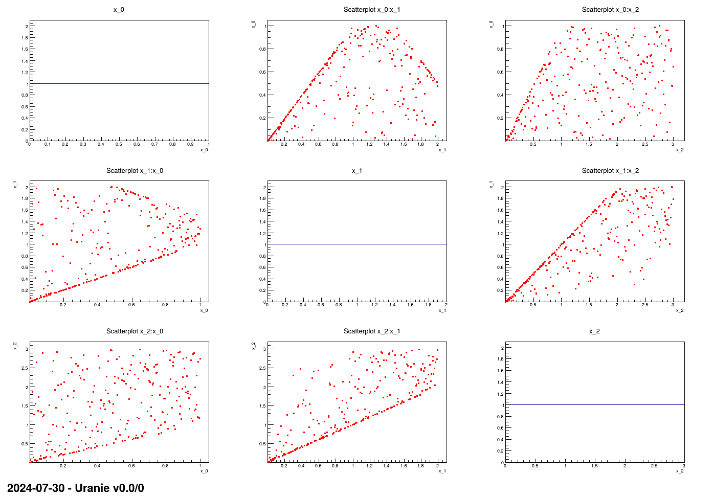
The idea behing this empirical heuristic is to rely on permutations and to decide on the best permutation to be done thanks to the content of the constraint matrix and also the distributions of solutions along the row and columns. This will be discussed further in the rest of this section but first a focus is done on the definition of a constraint. If one considerers a simple constraint, its implementation can be decompose in the following steps:
define it simply with an equation, for instance one wants to reject all locations for which
 ;
;
define a constraint function that can compute the margin of success, for instance in our simple case
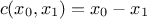 ;
;
define a characteristic constraint function that only states whether the constraint is fulfilled, for instance in our simple case
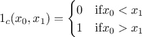
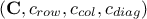
If formally the constraint function can provide more information when reading it (in terms of margin), one needs to know the way to apply a selection on these results which is not the simplest aspect to provide which explains why in the rest of this section the focus will be put on the characteristic contraint function. In order to illustrate our method, one can start from a provided LHS design-of-experiments, called hereafter
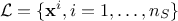
where
 is the i-Th
location which can be written as
is the i-Th
location which can be written as 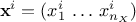 : it is a sample of size in the input space. From there, the constraint matrix is indeed defined as done
below:
: it is a sample of size in the input space. From there, the constraint matrix is indeed defined as done
below:
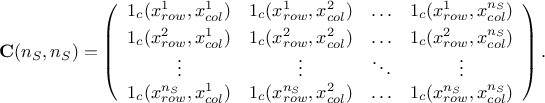
The constraint matrix is, as visible from the definition above, a  matrix which only contains 0 and 1 depending on whether the
current configuratio of the
matrix which only contains 0 and 1 depending on whether the
current configuratio of the  plane fulfill the constraint. This shows why restraining the constraint
to only two-variables function is a reasonable approach: for a given configuration the number of permutations will
blow up if one will considerer larger dimension constraint. Giving this object, one can introduces more useful
objects:
plane fulfill the constraint. This shows why restraining the constraint
to only two-variables function is a reasonable approach: for a given configuration the number of permutations will
blow up if one will considerer larger dimension constraint. Giving this object, one can introduces more useful
objects:
the constraint row solution vector, that sums up for every row the number of solutions, i.e. the number of columns that allow to fulfill the constraint
 ;
;
the constraint column solution vector, that sums up for every column the number of solutions, i.e. the number of row that allow to fulfill the constraint
 ;
;
the constraint diagonal vector i.e. the diagonal of the constraint matrix
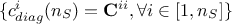 .
.
Bearing in mind that the objective is to have a constraint fulfilled, the heuristic will use the following criterion
as a stopping signal: 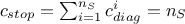 . This heuristic starts from a provided LHS design-of-experiments for which one can
consider three cases:
. This heuristic starts from a provided LHS design-of-experiments for which one can
consider three cases:
- A
it cannot fulfill the constraint, meaning that there is no sets of permutation to have
 ;
;
- B
it can fulfill the constraint with only one set of permutation leading to the only solution
 ;
;
- C
it can fulfill the constraint with many different sets of permutation leading to a very large number of configurations and so to a very large number of constrained design-of-experiments.
Practically, the heuristic is organised in a step-by-step approach in which the variable used as first argument in
the constraint definition will be used as row indicator (it will be called  ) and it is considered fixed. This implies that the permutation
will be done by reorganising the second variable, called
) and it is considered fixed. This implies that the permutation
will be done by reorganising the second variable, called  . The heuristic is then described below:
The constraint matrix is estimated along with all the objects discussed above
 .
.
If
 contains one 0, it means that the design-of-experiments cannot fulfill the constaint. If this design-of-experiments, has been provided,
the method stops, on the other hand if it was generated on-the-fly, then another attempt is done (up to
5 times).
contains one 0, it means that the design-of-experiments cannot fulfill the constaint. If this design-of-experiments, has been provided,
the method stops, on the other hand if it was generated on-the-fly, then another attempt is done (up to
5 times).
A bipartite graph method is called to check that there can be at least one solution for every row. If not, if the design-of-experiments has been provided, the method stops, on the other hand if it was generated on-the-fly, then another attempt is done (up to 5 times).
This step allows to sort out the design-of-experiments that will fall into the category A (defined above) from those that might fall either in the B or C ones.
If
 , then all the rows for which the diagonal elements
is 0 are kept aside and sorted out by increasing number of solutions over all the columns (their value of
, then all the rows for which the diagonal elements
is 0 are kept aside and sorted out by increasing number of solutions over all the columns (their value of
 ),
which defines
),
which defines 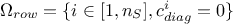 . The row considered, whose index will be written
k for kept hereafter, is the one with the lowest number of solutions (the most urgent one in a way), so it
can be written
. The row considered, whose index will be written
k for kept hereafter, is the one with the lowest number of solutions (the most urgent one in a way), so it
can be written 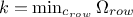
For
 the
chosen value, all the columns that provide a solution are kept aside and sorted out by increasing
order[5] of solutions over all rows (their value of
the
chosen value, all the columns that provide a solution are kept aside and sorted out by increasing
order[5] of solutions over all rows (their value of  ), which defines
  . This sorting provides information on the marging, as the highest
values of solutions over the rows means that this value of is compatible with many other instances. A loop is performed over all these
solutions, so that
. This sorting provides information on the marging, as the highest
values of solutions over the rows means that this value of is compatible with many other instances. A loop is performed over all these
solutions, so that  :
:
By definition we know that
 and
and  , so if then the
permutation will only increase the stopping criterion (), as the actual column
, so if then the
permutation will only increase the stopping criterion (), as the actual column  , will become the new column
 after
permutation. In this case, one can move to the permutation step. This can be written, by calling
after
permutation. In this case, one can move to the permutation step. This can be written, by calling
 the actual index of
the column (for selected),
the actual index of
the column (for selected),  . From there, one moves to the permutation step.
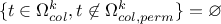
If none of the solution
under investigation can satisfy the requirement , then
 . In this definition, the ensemble
  is the ensemble of column index
which has already been used previously (as this is an interative heuristic) in a permutation for the
row under
investigation. This precaution has been introduced in order to prevent from having a loop in the
permutation process. From there, one moves to the permutation step.
is the ensemble of column index
which has already been used previously (as this is an interative heuristic) in a permutation for the
row under
investigation. This precaution has been introduced in order to prevent from having a loop in the
permutation process. From there, one moves to the permutation step.
If
 , meaning that all
possible solutions have been tested, then the selected column index is the result of a random drawing
in the nsemble of solutions, meaning that
, meaning that all
possible solutions have been tested, then the selected column index is the result of a random drawing
in the nsemble of solutions, meaning that  . From there, one moves to the
permutation step.
. From there, one moves to the
permutation step.
Now that both
and
are known, the
permutation will be done, it consists in:
changing content of the design-of-experiments, meaning doing
 ;
;
changing the columns in the constraint matrix, meaning doing
 ;
;
changing the content of the constraint column solution vector, meaning doing
 ;
;
fill once more the constraint diagonal vector (
 ) and compute once more the stopping criterion
() to
check whether the permutation process has to be continued. If so, then one moves to the second step.
) and compute once more the stopping criterion
() to
check whether the permutation process has to be continued. If so, then one moves to the second step.
This presentation has been simplified as, here, there is only one constraint applied to the design-of-experiments. Indeed, when
there are more than one constraint, let's call  and
and  the objects
associated to two constraints defined in both planes
the objects
associated to two constraints defined in both planes  and
and  , few cautions and extra steps have to be
followed as long as both stopping criteria,
, few cautions and extra steps have to be
followed as long as both stopping criteria,  or are different from depending on the variables in the constraint plane definition:
if planes
and have no common variable, or if
 but
but  then the constraints can be considered orthogonal;
if
 is the
same variable as
is the
same variable as  then any permutations for the constraint have to be propagated to the objects of the constraint , meaning that on top of the list in step
4, the extra steps consist in:
then any permutations for the constraint have to be propagated to the objects of the constraint , meaning that on top of the list in step
4, the extra steps consist in:
changing the rows in the constraint matrix for the constraint
, meaning doing  ;
;
changing the content of the constraint row solution vector for constraint
, meaning doing  ;
;
fill also the constraint diagonal vector (
 ) and compute once more the stopping criterion (
 ) to check whether the
permutation process has to be continued.
) to check whether the
permutation process has to be continued.
if
 , then any permutations from on the constraint can undo a previous one defined from the
other one, meaning that one can create a loop that will (thanks to our heuristic definition) will end up into
the random permutation area. To prevent this, so far, one can not create a second constraint using the same
variable as second argument.
, then any permutations from on the constraint can undo a previous one defined from the
other one, meaning that one can create a loop that will (thanks to our heuristic definition) will end up into
the random permutation area. To prevent this, so far, one can not create a second constraint using the same
variable as second argument.
| |  | |
| Chapter III. The Sampler module |  | III.3. QMC method |