

Documentation
/ Guide méthodologique
: 
| Chapter IV. Generating surrogate models | ||
|---|---|---|
 |  | |
Table of Contents
This part discusses the generation of
surrogate models which aim to provide a simpler, and hence faster, model in order to emulate the specified output of a more
complex model (and generally time and memory consuming) as a function of its inputs and parameters. The input dataset can either be an existing set of elements
(provided by someone else, resulting from simulations or experiments) or it can be a design-of-experiments generated on purpose, for
the sake of the ongoing study. This ensemble (of size  ) can be written as
 is the i-Th input vector which can be written as
  and
the output
and
the output  .
.
There are several predefined surrogate-models proposed in the Uranie platform:
The linear regression, discussed in Section IV.2
The chaos polynomial expansion, discussed in Section IV.3
The artificial neural networks, discussed in Section IV.4
The Kriging method, or gaussian process, discussed in Section IV.5
It is recommended to follow the law of parsimony (also called Ockham's razor) meaning that the simplest model should be
tested first, unless one has insight that it is not well suited for the problem under consideration. There have been many analysis performed to try to provide better guideline than the Ockham's razor on
what model to choose, knowing a bit about the physical problem under study. Among these, one can look at this reference
[Simpson2001] that proposes the following recommendations:
Polynomial models: well-established and easy to use, they are best suited for applications with random error and
appropriate for applications with <10 factors.
Neural networks: good for highly nonlinear or very large problems (
Kriging: extremely flexible but complex, they are well-suited for deterministic applications and can handle
applications with <50 factors.
 10 000 parameters), they might be best suited for deterministic
applications but they imply high computational expense (often .10,000 training data points); best for repeated
application.
10 000 parameters), they might be best suited for deterministic
applications but they imply high computational expense (often .10,000 training data points); best for repeated
application.
As already stated previously, surrogate models rely on a training database  whose size should be sufficient to allow a proper estimation of the hyper-parameters, providing
a nice estimation of the quantity of interest. The next two parts will introduce the concept of quality criteria and
the basic problem of under- and over-fitting.
whose size should be sufficient to allow a proper estimation of the hyper-parameters, providing
a nice estimation of the quantity of interest. The next two parts will introduce the concept of quality criteria and
the basic problem of under- and over-fitting.
Once the model hyper-parameters are set (this step depends heavily on the chosen model, as discussed in the rest of
this section), the quantity of interest can be estimated as  , where
  represents the surrogate model. Only using the training database
, one can have a
first hint on whether this estimation can be considered reliable or not, thanks to various quality criteria. Among
these, one can state for instance
represents the surrogate model. Only using the training database
, one can have a
first hint on whether this estimation can be considered reliable or not, thanks to various quality criteria. Among
these, one can state for instance

where 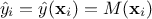 is the prediction from the surrogate model at the i-Th location and
 is the
expectation of the true value of our quantity of interest under consideration. MSE stands for Mean Square
Error and should be as close to 0 as possible. The
is the
expectation of the true value of our quantity of interest under consideration. MSE stands for Mean Square
Error and should be as close to 0 as possible. The  coefficient on the other hand should as close to 1 as possible to state that the
model might be valid. The last coefficient is just the "adjusted" , to regularise the fact that tends to be artificially close to 1 when the input space
dimension
coefficient on the other hand should as close to 1 as possible to state that the
model might be valid. The last coefficient is just the "adjusted" , to regularise the fact that tends to be artificially close to 1 when the input space
dimension  is large. A final
caveat about MSE: unlike ,
MSE is not "scaled" or "normalised", so if one is dealing with a model whose results are small numerically, the
surrogate model might be very wrong while having a small MSE. The scaling performed when computing (dividing by the variance of the true
model) is coping for this.
is large. A final
caveat about MSE: unlike ,
MSE is not "scaled" or "normalised", so if one is dealing with a model whose results are small numerically, the
surrogate model might be very wrong while having a small MSE. The scaling performed when computing (dividing by the variance of the true
model) is coping for this.
The criteria discussed above are only using the training database and their interpretation can be misleading in case of
over-fitting for instance (see Section IV.1.2 for a discussion on this matter). To prevent
this, it is possible to use another database, often called validation database[6] that will be called
hereafter  and
whose size is
and
whose size is  . The
predictivity coefficient
. The
predictivity coefficient  is
analogous to the one, as one
can write
is
analogous to the one, as one
can write
The data are this time coming from the validation
database ( so they have not been used to train de surrogate
model. The closer to 1 the
coefficient is, the more predictive the model can be considered.
so they have not been used to train de surrogate
model. The closer to 1 the
coefficient is, the more predictive the model can be considered.
Finally, for some surrogate models only, it is possible to perform a certain type of cross-validation for no or very
limited cost. The idea is to obtain the prediction 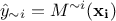 where
where  represents the surrogate model for which
the training database would have been without the i-Th location (
represents the surrogate model for which
the training database would have been without the i-Th location ( is therefore called the Leave-one-out
prediction). The resulting quality criteria are then defined as
is therefore called the Leave-one-out
prediction). The resulting quality criteria are then defined as

This happen to be very practical when
the data are rare and expensive to produce: it is indeed complicated to "sacrifice" good data to test the validity.
This part describes the possible problem that one can meet when trying to train a surrogate model. Starting back from
the situation described previously where and are respectively our training and validation database. If one assumes that the
following relation  can exist (basically introducing a white noise
  ,
then finding a proper surrogate model would mean finding the "function"
,
then finding a proper surrogate model would mean finding the "function"  that can generalise to location out of the training database and whose
error on the validation database can be written as:
that can generalise to location out of the training database and whose
error on the validation database can be written as:
This total error is the sum of three different contributions :
an irreducible error,
 , which is the lowest limit expected on a validation test;
a bias term,
 , which is the difference between the average prediction of our model and
the correct value, that we are trying to predict;
, which is the difference between the average prediction of our model and
the correct value, that we are trying to predict;
a variance term,
 , which is the variability of our model prediction for a given data point or
a value, that tells us spread of our data.
, which is the variability of our model prediction for a given data point or
a value, that tells us spread of our data.
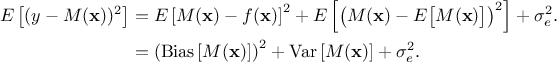
Getting the best surrogate model is then a minimisation of both the variance and bias term, even though usually these two criteria are antagonist: the more complex the surrogate model is, the smaller the bias is becoming. Unfortunately, this reduction of the bias goes with an increase of the variance as the model tends to adapt itself more to the data. This is known as the "Variance-Bias dilemma" or the "Variance-Bias trade-off". This is sketched in Figure IV.1 that depicts the evolution of the bias, the variance and their sum, as a function of the complexity of the model.
Figure IV.1. Sketch of the evolution of the bias, the variance and their sum, as a function of the complexity of the model.
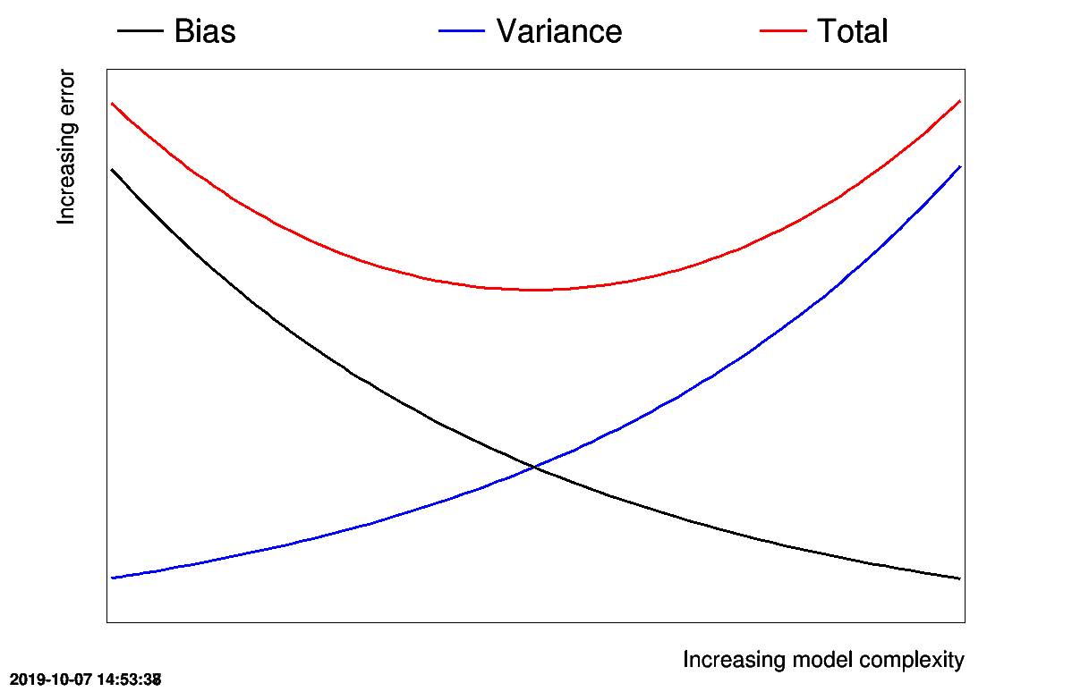 |
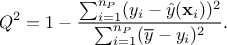
There are usually three situations that one can come across when dealing with surrogate models, all depicted in Figure IV.2, where black and yellow dots respectively represent a training and a validation database. The ideal situation is the third one, in the right-hand side of the figure, where the green line passes in between all points, meaning that the model predictions are close to all original values, disregarding the database they're coming from. This leads to a low bias and, as the variations are smooth and small through the entire range, a low variance as well. Let's now discuss the two other situations.
Figure IV.2. Sketches of under-trained (left), over-trained (middle) and properly trained (right) surrogate models, given that the black points show the training database, while the yellow ones show the testing database
 |
The first situation, shown in the left part Figure IV.2, is what is called under-fitting: the model cannot capture the proper behaviour of the code and if one wants to estimate the MES, either for the training or validation database, the result in both cases will be poor. It generally arises when one assumes an over-simplified model either because of a lack of data or because of a mis-knowledge of the general trend of the problem under consideration. On the validation database, the prediction coming from the blue line will have an obvious low (null) variance and mainly a large bias (which is characteristic of under-fitting issue).
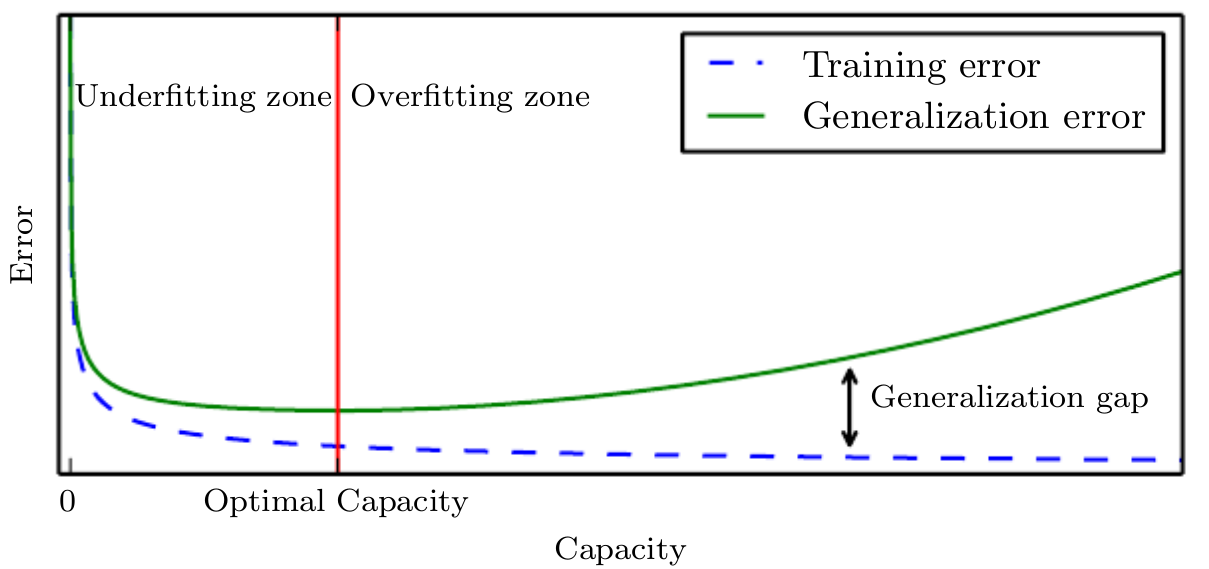
The opposite situation, represented in red in the middle of Figure IV.2, is what is called over-fitting: the model has learned (almost perfectly) the training database, and only it. It failed in capturing the proper trend of the code and if one applies this model to a validation database, the resulting prediction will be really poor. This situation corresponds to the case where the variance is becoming large. There are several strategies to avoid being in the situation but in general the first thing to check is that there is consistency between the the degrees of freedom of the model and the degree of freedom provided through the training database. One of the possible mechanism consists, for instance, in splitting the training database into a large sub-part used to train the model and a smaller one used to control how well the resulting model can predict unknown points. If one computes and represents the MSE for both sub-parts, as a function of the training steps, the resulting curves should look as those depicted in Figure IV.3. On the first hand, the MSE estimated on the training sub-part only gets better along the training, while on the other hand, the MSE computed on the control sample (called generalisation error, as it represents how well the model can be generalised to the rest of the input space) diminishes along the training error up to a plateau and then it grows again. This plateau is where one should stop the training procedure.
Figure IV.3. Evolution of the different kinds of error used to determine when does one start to over-train a model
 |
| | | |
| III.3. QMC method |  | IV.2. The linear regression |