

Documentation
/ Methodological guide
: 
| IV.3. Chaos polynomial expansion | ||
|---|---|---|
 | Chapter IV. Generating surrogate models |  |
The concept of polynomial chaos development relies on the homogeneous chaos theory introduced by Wiener in 1938
[Wiener38] and further developed by Cameron and Martin in 1947
[Cameron47]. Using polynomial chaos (later referred to as PC ) in
numerical simulation has been brought back to the light by Ghanem and Spanos in 1991
[Ghanem91]. The basic idea is that any square-integrable function can be written as
 where
where  are the PC coefficients,
  is the orthogonal
polynomial-basis. The index over which the sum is done,
is the orthogonal
polynomial-basis. The index over which the sum is done,  , corresponds to a multi-index whose dimension is equal to the dimension of
vector
, corresponds to a multi-index whose dimension is equal to the dimension of
vector  (i.e.
(i.e.  )
and whose L1 norm (
)
and whose L1 norm ( ) is the degree of the resulting polynomial. Originally written to deal
with normal law, for which the orthogonal basis is Hermite polynomials, this decomposition is now generalised to
few other distributions, using other polynomial orthogonal basis (the list of those available in Uranie is shown
in Table IV.1).
) is the degree of the resulting polynomial. Originally written to deal
with normal law, for which the orthogonal basis is Hermite polynomials, this decomposition is now generalised to
few other distributions, using other polynomial orthogonal basis (the list of those available in Uranie is shown
in Table IV.1).
Table IV.1. List of best adapted polynomial-basis to develop the corresponding stochastic law
| Distribution \ Polynomial type | Legendre | Hermite | Laguerre | Jacobi |
|---|---|---|---|---|
| Uniform | X | |||
| LogUniform | X | |||
| Normal | X | |||
| LogNormal | X | |||
| Exponential | X | |||
| Beta | X |
This decomposition can be helpful in many ways: it can first be used as a surrogate model but it gives also access,
through the value of its coefficient, to the sensitivity index (this will be first introduced in Section IV.3.1.2 and further developed in Chapter V).
We'll discuss here a simple example of polynomial chaos development and its implication. In the case where a system
is depending on two random variables,  and
and  that
follow respectively an uniform and normal distribution, giving rise to a single output
that
follow respectively an uniform and normal distribution, giving rise to a single output  . Following the remark about square-integrable functions,
both inputs can be decomposed on a specific orthogonal polynomial-basis, such as
. Following the remark about square-integrable functions,
both inputs can be decomposed on a specific orthogonal polynomial-basis, such as  ,
and
,
and  , where
  and
and  are the PC coefficients that respectively multiply the
Legendre (
are the PC coefficients that respectively multiply the
Legendre ( ) and
Hermite (
) and
Hermite ( )
polynomials, for the uniform and normal law and where is the multi-index (here of dimension 1) over which the sum is done. These basis
are said to be orthogonal because for any degrees
)
polynomials, for the uniform and normal law and where is the multi-index (here of dimension 1) over which the sum is done. These basis
are said to be orthogonal because for any degrees  and
and  , taking the Legendre case as an example, one can write
 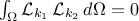 , for
, for  .
.
It is now possible to write the output, , as a function of these polynomials. For the  -Th simulation,
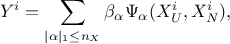
where is the multi-index of dimension 2 ( ) over which the sum is performed. The
  polynomials are built by tensor products of the inputs basis following the
previously defined degree. In the specific case of the simple example discussed here, this leads to a decomposition
of the output that can be written as
polynomials are built by tensor products of the inputs basis following the
previously defined degree. In the specific case of the simple example discussed here, this leads to a decomposition
of the output that can be written as
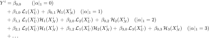
From this development, it becomes clear that a
threshold must be chosen on the order of the polynomials used, as the number of coefficient is growing quickly,
following this rule 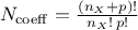 , where
  is the cut-off chosen on the polynomial degree. In this example, if we choose to use
 , this leads to only 6
coefficients to be measured:
, this leads to only 6
coefficients to be measured:  . Their
estimation is discussed later.
. Their
estimation is discussed later.
These coefficients are characterising the surrogate model and can be used, when the inputs are independent, to estimate the corresponding Sobol's coefficients (a deeper discussion about these coefficients and their meaning can be found in Section V.1). For the uniform and normal example, the first order coefficients are respectively given by
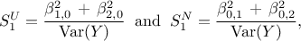
whereas the total order coefficients are respectively given by
The complete variance of the output, can also be written as
Warning
One can use chaos polynomial expansion with a training database without knowing the probability laws used to
generate it, as long as the polynomial coefficients estimation is done with a regression method and not an
integration one (for which the integration-oriented design-of-experiments is made specifically knowing the laws, see discussion
in Section IV.3.2.1 and Section IV.3.2.2).
The
interpretation of the polynomial coefficients as Sobol's coefficients, on the other hand, is
strongly relying on the hypothesis that the probability laws have been properly defined, so it becomes not
suitable if the training database is made without knowing the probability laws. The explanations for this is way
beyond the scope of this documentation but more information can be found in the literature (for instance in
[roustant2019sensitivity]).
The wrapper of the Nisp library, Nisp standing for Non-Intrusive Spectral Projection, is a tool allowing to access to Nisp functionality from the Uranie platform. The main features are detailed below.
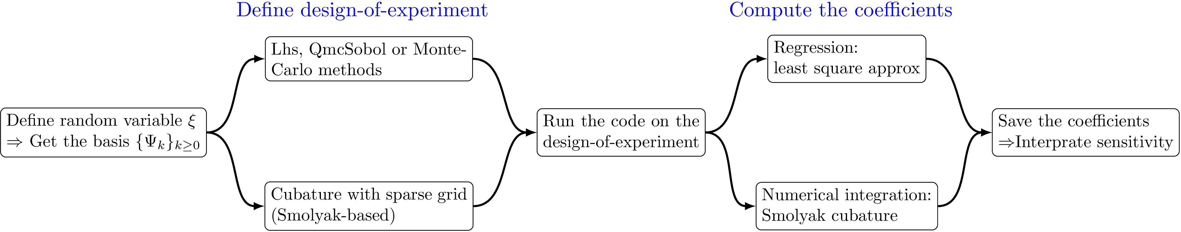
The Nisp library [baudininria-00494680] uses spectral methods based on polynomial chaos in order to provide a surrogate model and allow the propagation of uncertainties if they arise in the numerical models. The steps of this kind of analysis, using the Nisp methodology are represented schematically in Figure IV.5 and are introduced below:
Specification of the uncertain parameters xi,
Building stochastic variables associated xi,
Building a design-of-experiments
Building a polynomial chaos, either with a regression or an integration method (see Section IV.3.2.1 and Section IV.3.2.1)
Uncertainty and sensitivity analysis
The regression method is simply based on a least-squares approximation: once the design-of-experiments is done, the vector of
output  is
computed with the code. The regression coefficients
is
computed with the code. The regression coefficients  are estimated considering that every computed output points
can be represented following Equation IV.5. By writing the correspondence matrix
are estimated considering that every computed output points
can be represented following Equation IV.5. By writing the correspondence matrix
 and the
coefficient-vector
and the
coefficient-vector  , this estimation is just a minimisation of
  , where, once back to our simple example from Section IV.3.1.2 for illustration purpose, As
already stated in Section IV.2, this leads to write the general form of the solution
as
, where, once back to our simple example from Section IV.3.1.2 for illustration purpose, As
already stated in Section IV.2, this leads to write the general form of the solution
as 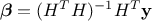 which also shows that the way the design-of-experiments is performed can be optimised
depending on the case under study (and might be of the utmost importance in some rare case).
which also shows that the way the design-of-experiments is performed can be optimised
depending on the case under study (and might be of the utmost importance in some rare case).
In order to perform this estimation, it is mandatory to have more points in the design-of-experiments than the number of
coefficient to be estimated (in principle, following the rule  leads to a safe estimation).
The integration method relies on a more "complex" design-of-experiments. It is indeed recommended to have dedicated design-of-experiments, made
with a Smolyak-based algorithms (as the ones cited in Figure IV.5). These design-of-experiments are
sparse-grids and usually have a smaller number of points than the regularly-tensorised approaches. In this case,
the number of samples has not to be specified by the user. Instead, the argument requested describes the level of
the design-of-experiments (which is closely intricated, as the higher the level is, the larger the number of samples is). Once this
is done, the calculation is performed as a numerical integration by quadrature methods, which requires a large
number of computations.
In the case of Smolyak algorithm, this number can be expressed by the number of
dimensions and the requested
level  as
as 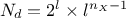 which shows an
improvement with respect to the regular tensorised formula for quadrature (
which shows an
improvement with respect to the regular tensorised formula for quadrature ( ).
).
| |  | |
| IV.2. The linear regression |  | IV.4. The artificial neural network |