

Documentation
/ Methodological guide
: 
| IV.4. The artificial neural network | ||
|---|---|---|
 | Chapter IV. Generating surrogate models |  |
The Artificial Neural Networks (ANN) in Uranie are Multi Layer Perceptron
(MLP) with one or more hidden layer (containing  neurons, where
  is use to identify the layer) and one or more output variable.
The concept of formal neuron, has been proposed in 1943, after observing the way biological neurons are intrinsically connected [McCulloch1943]. This model is a simplification of the various range of functions dealt by a biological neuron, the formal one (displayed in Figure IV.6) being requested to satisfy only the two following:
summing the weighted input values, leading to an output value called neuron's activity
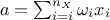 ,
where
,
where  are the synaptic weights of the neuron.
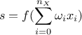
emitting a signal (whether the output level goes beyond a chosen threshold or not)
 where
where  and
and  are respectively the transfer function and the bias of
the neuron.
are respectively the transfer function and the bias of
the neuron.
Figure IV.6. Schematic description of a formal neuron, as seen in McCulloch and Pitts [McCulloch1943].
![Schematic description of a formal neuron, as seen in McCulloch and Pitts [McCulloch1943].](https://uranie.cea.fr/images/neurone.png) |
One can introduce a shadow input defined as  (or -1), which lead to consider the bias as another synaptic weight
 . The
resulting emitted signal is written as
. The
resulting emitted signal is written as
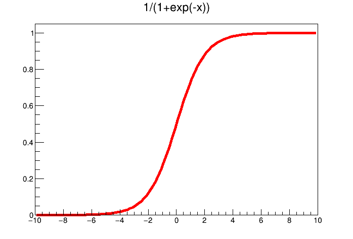
There are a large variety of transfer
functions possible, and an usual starting point is the sigmoid family, defined with three real parameters, c, r and
k, as 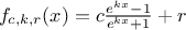 . Setting these parameters to peculiar values leads to known functions as the
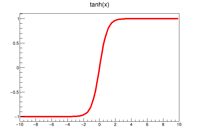
hyperbolic tangent and the logistical function, shown in Figure IV.7 and defined as
. Setting these parameters to peculiar values leads to known functions as the
hyperbolic tangent and the logistical function, shown in Figure IV.7 and defined as

Figure IV.7. Example of transfer functions: the hyperbolic tangent (left) and the logistical one (right)
The artificial neural network conception and
working flow has been first proposed in 1962 [rosenblatt196] and was called the
perceptron. The architecture of a neural network is the description of the organisation of the formal neurons and the
way they are connected together. There are two main topologies:
Figure IV.8. Schematic description of the working flow of an artificial neural network as used in Uranie
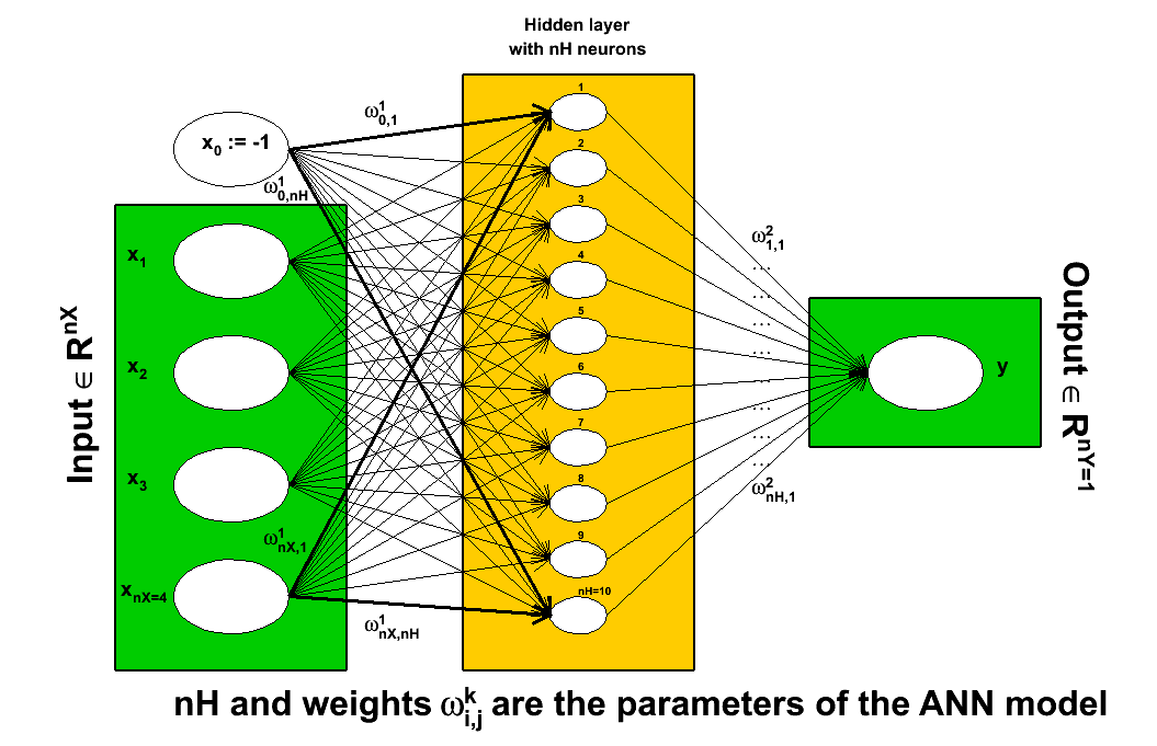 |
The first step is the definition of the problem: what are the input variables under study, how many neurons will be
created in how many hidden layers, what is the chosen activation function. When choosing the architecture of an
artificial neural network, one should keep in mind that the number of points used to perform the training should
obviously be greater than the number of parameters to be estimated, i.e. the number of synaptic
weights (the usual rule of thumb being having a factor 1.5 between data points and the number of coefficients). From
the explanation given previously, the number of coefficients for a single hidden layer neural network is 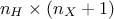 where
where
 is the number of neurons
chosen. This formula can be generalised to multi-layer cases, as
is the number of neurons
chosen. This formula can be generalised to multi-layer cases, as
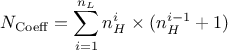
In this equation, is the number of hidden neurons per layer, for  where
where  is the number of layer, and
  is the number of inputs (
 ). Defining an
architecture is quite tricky and depends on the problem under consideration. Going multi-layer is a way to reduce the
number of coefficients to be estimated when the number of inputs is large: with 9 inputs variables, a mono-layer with
8 neurons will have 80 synaptic weights while a network with 3 layers and 3 neurons each, will have 9 neurons in
total but only 54 weights to be determined.
). Defining an
architecture is quite tricky and depends on the problem under consideration. Going multi-layer is a way to reduce the
number of coefficients to be estimated when the number of inputs is large: with 9 inputs variables, a mono-layer with
8 neurons will have 80 synaptic weights while a network with 3 layers and 3 neurons each, will have 9 neurons in
total but only 54 weights to be determined.
The second step is the training of the ANN. This step is crucial and many different
techniques exist to achieve it but, as this note is not supposed to be exhaustive, only the one considered in the
Uranie implementation will be discussed. A learning database should be provided, composed of a set of inputs and
the resulting output (the ensemble
the learning itself. By varying all the synaptic weights contained in the parameter From there, one can define the risk function
the regularisation. This step is made to avoid all over-fitting problem, meaning that the neural network would
be trained only for the  discussed in Section IV.1). From that, two mechanisms are run simultaneously:
 , the aim is to produce the
output set
, the aim is to produce the
output set  , that would be as close as possible to the output stored in
and keep the
best configuration (denoted as
, that would be as close as possible to the output stored in
and keep the
best configuration (denoted as  ). The difference between the real outputs and the estimated ones are
measured through a loss function which could be, in the case of regression, a quadratic loss function such as
). The difference between the real outputs and the estimated ones are
measured through a loss function which could be, in the case of regression, a quadratic loss function such as
 (also
called cost or energy function) used to transform the optimal parameters search into a minimisation problem.
The empirical risk function can indeed be written as
(also
called cost or energy function) used to transform the optimal parameters search into a minimisation problem.
The empirical risk function can indeed be written as  ensemble which might not be representative of the rest of the input space. To avoid this, the
learning database is split into two sub-parts: one for the learning as described in the previous item, and one
to prevent the over-fitting to happen. This is done by computing for every newly tested parameter set , the generalised error
(computed as the average error over the set of points not used in the learning procedure). While it is expected
that the risk function is becoming smaller when the number of optimisation step is getting higher, the generalised
error is also becoming smaller at first, but then it should stabilise and even get worse. This flattening or
worsening is used to stop the optimisation.
ensemble is done using a random generator, so does the initialisation of the
synaptic weights for all the formal neurons.
ensemble which might not be representative of the rest of the input space. To avoid this, the
learning database is split into two sub-parts: one for the learning as described in the previous item, and one
to prevent the over-fitting to happen. This is done by computing for every newly tested parameter set , the generalised error
(computed as the average error over the set of points not used in the learning procedure). While it is expected
that the risk function is becoming smaller when the number of optimisation step is getting higher, the generalised
error is also becoming smaller at first, but then it should stabilise and even get worse. This flattening or
worsening is used to stop the optimisation.
ensemble is done using a random generator, so does the initialisation of the
synaptic weights for all the formal neurons.
Finally, the constructed neural network can be (and should be) exported: the weight initialisation, but also the way the split is performed between the test and training basis, are randomised leading to different results every time one redo the training procedure.
| |  | |
| IV.3. Chaos polynomial expansion |  | IV.5. The kriging method |