

Documentation
/ Methodological guide
: 
| IV.5. The kriging method | ||
|---|---|---|
 | Chapter IV. Generating surrogate models |  |
First developed for geostatistic needs, the kriging method, named after D. Krige and also called Gaussian Process method (denoted GP hereafter) is another way to construct a surrogate model. It recently became popular thanks to a series of interesting features:
it provides a prediction along with its uncertainty, which can then be used to plan the simulations and therefore improve the predictions of the surrogate model
it relies on relatively simple mathematical principle
some of its hyper-parameters can be estimated in a Bayesian fashion to take into account a priori knowledge.
Kriging is a family of interpolation methods developed in the 1970s for the mining industry [Matheron70]. It uses information about the "spatial" correlation between observations to make predictions with a confidence interval at new locations. In order to produce the prediction model, the main task is to produce a spatial correlation model. This is done by choosing a correlation function and search for its optimal set of parameters, based on a specific criterion.
The gpLib library [gpLib] provides tools to achieve this task. Based on the gaussian process properties of the kriging [bacho2013], the library proposes various optimisation criteria and parameter calculation methods to find the parameters of the correlation function and build the prediction model.
The present chapter describes the integration of the gpLib inside Uranie, from a methodological point of view. For a more practical point of view, see the gpLib tutorial [KrigUranie].
The modelisation relies on the assumption that the deterministic output  can be written as a realisation of a gaussian process
 that can be
decomposed as
that can be
decomposed as  where
where  is the deterministic part that describes the expectation of the process and
 is the
stochastic part that allows the interpolation. This method can also take into account the uncertainty coming from the
measurements. In this case, the previously-written is referred to as
is the
stochastic part that allows the interpolation. This method can also take into account the uncertainty coming from the
measurements. In this case, the previously-written is referred to as  and the gaussian process is then decomposed into
 , where
  is the uncertainty
introduced by the measurement.
is the uncertainty
introduced by the measurement.
The first step is to construct the model from the  known measurements, that will be hereafter called the training site. To do so, a parametric
correlation function has to be chosen amongst a list of provided one (discussed in Section IV.5.1.1); a deterministic trend can also be imposed to bring more information on the
behaviour of the output expectation. These steps define the list of hyper-parameters to be estimated, which is done in
Uranie through an optimisation loop. The training site and the estimated hyper-parameters constitute the kriging
model that can then be used to predict the value of a new sets of points.
known measurements, that will be hereafter called the training site. To do so, a parametric
correlation function has to be chosen amongst a list of provided one (discussed in Section IV.5.1.1); a deterministic trend can also be imposed to bring more information on the
behaviour of the output expectation. These steps define the list of hyper-parameters to be estimated, which is done in
Uranie through an optimisation loop. The training site and the estimated hyper-parameters constitute the kriging
model that can then be used to predict the value of a new sets of points.
It is possible, at this stage, even before applying the kriging model to a new set of points, to make a verification of
the covariance function at hand. This is done in Uranie using a Leave-One-Out (LOO)
technique. This method consists in the prediction of a value for  using the rest of the known values in the training site, i.e.
 for
for  . From there, it is possible to use the LOO prediction
  and the expectation
 to estimate both the
 and
and  (see Section IV.1.1 for completeness). The first criterion should be close to 0 while, if the covariance function is
correctly specified, the second one should be close to 1. Another possible test to check whether the model seems
reasonable consists in using the predictive variance vector
(see Section IV.1.1 for completeness). The first criterion should be close to 0 while, if the covariance function is
correctly specified, the second one should be close to 1. Another possible test to check whether the model seems
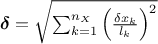
reasonable consists in using the predictive variance vector  to look at the distribution of the ratio
  for every point
in the training site. A good modelling should result in a standard normal distribution, so one can find in the
literature (see [jones98EGO] for instance) quality criteria proposal such as having at least 99.7%
of the points comply with
for every point
in the training site. A good modelling should result in a standard normal distribution, so one can find in the
literature (see [jones98EGO] for instance) quality criteria proposal such as having at least 99.7%
of the points comply with
The next section will introduce the correlation functions implemented, that can be used to learn from the data and set
the value of the corresponding hyper-parameters. This is a training step which should lead to the construction of the
covariance matrix  of the
stochastic part
introduced previously. From there, the predictions to new points can be performed, as discussed in Section IV.5.1.2.
of the
stochastic part
introduced previously. From there, the predictions to new points can be performed, as discussed in Section IV.5.1.2.
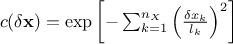
To end this introduction it might be useful to introduce one of the most used correlation function (at least a
very-general one): the Matern function. It uses the Gamma function  and the modified Bessel function of order
  called hereafter
  . This parameter describes the regularity (or smoothness) of the trajectory (the larger it
is, the smoother the function will be) which should be greater than 0.5. In one dimension, with
. This parameter describes the regularity (or smoothness) of the trajectory (the larger it
is, the smoother the function will be) which should be greater than 0.5. In one dimension, with  the distance, this function can be
written as
the distance, this function can be
written as
In this function,
 is the correlation length
parameter, which has to be positive. The larger is, the more
is the correlation length
parameter, which has to be positive. The larger is, the more  is correlated between two fixed locations
  and
and  and
hence, the more the trajectories of vary slowly with respect to
and
hence, the more the trajectories of vary slowly with respect to  .
As discussed in Section IV.5.1 this is a crucial part to specify a GP and there are many possible
functions implemented in Uranie. In the following list, are the correlation lengths and are the regularity parameters. For the rest of this discussion, the variance
parameter
.
As discussed in Section IV.5.1 this is a crucial part to specify a GP and there are many possible
functions implemented in Uranie. In the following list, are the correlation lengths and are the regularity parameters. For the rest of this discussion, the variance
parameter  will be
glossed over as it will be determined in all case and it is global (one value for a problem disregarding the number
of input variable). The impact of these parameters, variance, correlation length and smoothness are displayed
respectively in Figure IV.9, Figure IV.10and Figure IV.11 (these plots are taken from [bacho2013]).
will be
glossed over as it will be determined in all case and it is global (one value for a problem disregarding the number
of input variable). The impact of these parameters, variance, correlation length and smoothness are displayed
respectively in Figure IV.9, Figure IV.10and Figure IV.11 (these plots are taken from [bacho2013]).
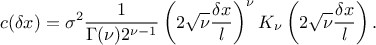
Figure IV.9. Influence of the variance parameter in the Matern function once fix at 0.5, 1 and 2 (from left to right). The correlation length is set to 1 while the smoothness is set to 3/2.
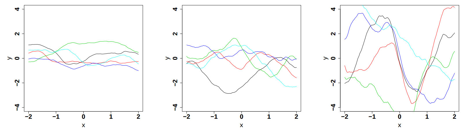 |
Figure IV.10. Influence of the correlation length parameter in the Matern function once fix at 0.5, 1 and 2 (from left to right). The variance is set to 1 while the smoothness is set to 3/2.
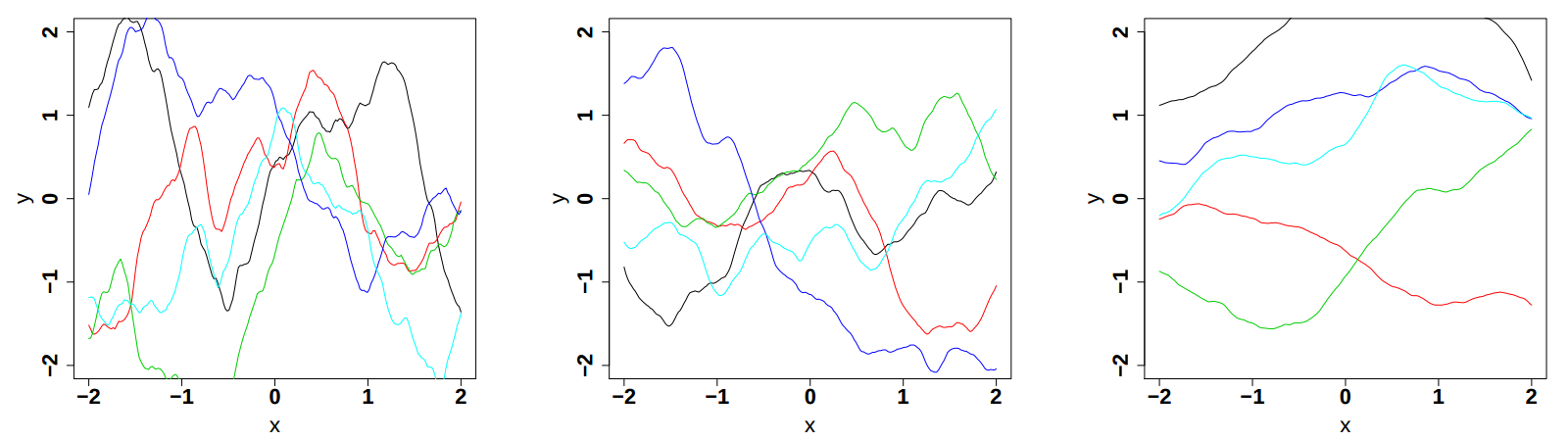 |
Figure IV.11. Influence of the smoothness parameter in the Matern function once fix at 0.5, 1.5 and 2.5 (from left to right). Both the variance and the correlation length are set to 1.
 |
Gauss: it is defined with one parameter per dimension, as
 .
.Isogauss: it is defined with one parameter only, as
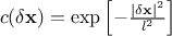 .
.Exponential: it is defined with two parameters per dimension, as
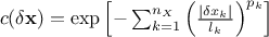 , where
  are the power parameters. If
  , the function is equivalent to the Gaussian correlation
function.
, the function is equivalent to the Gaussian correlation
function.MaternI: the most general form, it is defined with two parameters per dimension, as
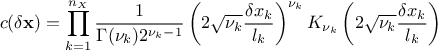
MaternII: it is defined as maternI, with only one common smoothness (leading to
 parameters).
 MaternIII: it first compute a distance as
 and then use Equation IV.6 with
  (leading to
parameters).
(leading to
parameters). Matern1/2: it is equivalent to maternIII, when

Matern3/2: it is equivalent to maternIII, when

Matern5/2: it is equivalent to maternIII, when

Matern7/2: it is equivalent to maternIII, when

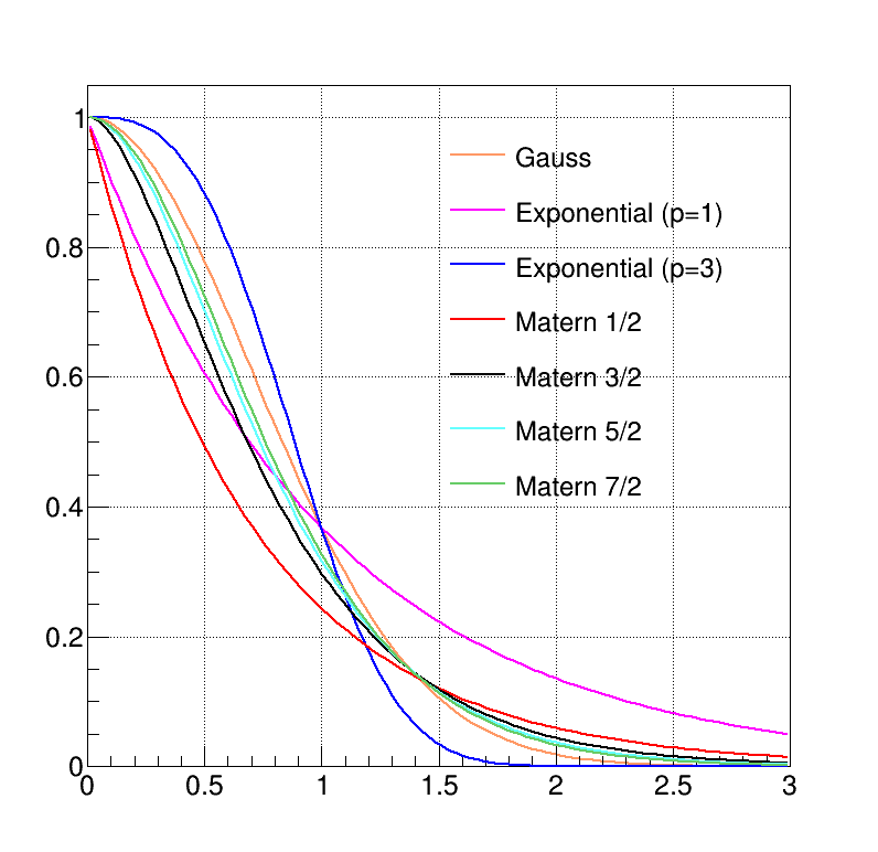
The choice has to be made on a case-by-case basis, knowing the behaviour of the various inputs along with the way the
output evolves. A gaussian function is infinitely derivable, so it is expected to work particularly well for cases
where the output has a smooth trend, whereas the exponential, when considering small powers,
i.e.  for instance, could better describe a more erratic output behaviour. The Matern function can easily
go from one of this performance to the other by changing the smoothness. Figure IV.12
presents the evolution of the different covariance functions implemented in Uranie.
for instance, could better describe a more erratic output behaviour. The Matern function can easily
go from one of this performance to the other by changing the smoothness. Figure IV.12
presents the evolution of the different covariance functions implemented in Uranie.
The predictions are done after the estimations of the hyper-parameters  of the covariance process, along with the
errors if this is requested and the trend parameters as-well. As a reminder, the probabilistic model is depicted as
of the covariance process, along with the
errors if this is requested and the trend parameters as-well. As a reminder, the probabilistic model is depicted as

where
 and
and  is a gaussian process independent from
  , possibly including uncertainty measurements. As already stated, is the covariance matrix of the stochastic part
 and
and  the gaussian vector defined as
  . For the sake of
simplicity, we will discuss only deterministic trend here where are supposed constant and are estimated from the regressor matrix
. For the sake of
simplicity, we will discuss only deterministic trend here where are supposed constant and are estimated from the regressor matrix
 , constructed from the
 , as already discussed in Section IV.2. For
a more general discussion on a bayesian approach to define the trend, see [bacho2013].
, as already discussed in Section IV.2. For
a more general discussion on a bayesian approach to define the trend, see [bacho2013].
Every prediction of the gaussian process at a new location  can be calculated from the conditional gaussian law
  which can be easily obtained from the joined law
  using the gaussian conditioning theorem[8]. Starting from the simple case where one wants to get the best estimate
  and its conditional
variance
and its conditional
variance  for a single new location . Both quantities can be expressed from the previous
matrix, using
for a single new location . Both quantities can be expressed from the previous
matrix, using  the regressor vector estimated at this new location and
  the vector (of
size ) of covariance computed
between this new location and the training set. The results are provided by the following equations:
the vector (of
size ) of covariance computed
between this new location and the training set. The results are provided by the following equations:
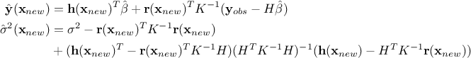
In the case where multiple locations have to be estimated and one wants to keep track of their possible correlation,
a more complex formula is written, starting from Equation IV.7. The regressor vector is now
written as  , a
regressor matrix gathering all new locations estimation,
, a
regressor matrix gathering all new locations estimation,  is a
is a  matrix that gathers covariance computed between all new locations and the
training set and finally
matrix that gathers covariance computed between all new locations and the
training set and finally  is introduced as the covariance matrix between all the new input locations (with a given size
 ). The results are then provided by the following equations:

The main interest of the second procedure is to provided the complete covariance matrix of the estimation so if one wants to investigate the residuals, when dealing with a validation database, the possible correlation between location can be taken into account (through a whitening procedure for instance, that is partly introduced in Section III.2.2) to have proper residuals distribution. There are different ways to that, see [bastos2009diagnostics], the ones used here are either based on Cholesky decomposition or eigen-value decomposition.
Finally, one interesting thing to notice is the fact that the prediction estimation needs both the inverse of the
covariance matrix  and the regressor matrix . This
means that with a large training database, this would mean keep this possibly two large matrices for every single new
location.
and the regressor matrix . This
means that with a large training database, this would mean keep this possibly two large matrices for every single new
location.
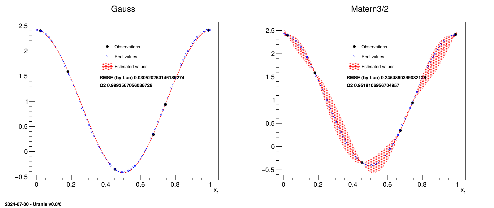
We illustrate the kriging method on a very simple model, i.e. an uni-dimensional function, and
display the resulting kriging model prediction. We use a training site with 6 points along with a test basis that
is made of about 100 points. The covariance function used is a Gaussian one (left) and a Matern one (right),
precisely a Matern3/2, presented in Figure IV.13. In this figure, one can see the training
sites (the six black points), the real values of the testing site (the blue crosses), the predicted value from the
kriging model (the red line) and the uncertainty band on this prediction (the red-shaded band). Both the MSE and
from LOO are also
indicated showing that in this particular case, the Gaussian choice is better than the Matern one.
Figure IV.13. Example of kriging method applied on a simple uni-dimensional function, with a training site of six points, and tested on a basis of about hundred points, with either a gaussian correlation function (left) or a matern3/2 one (right).
 |
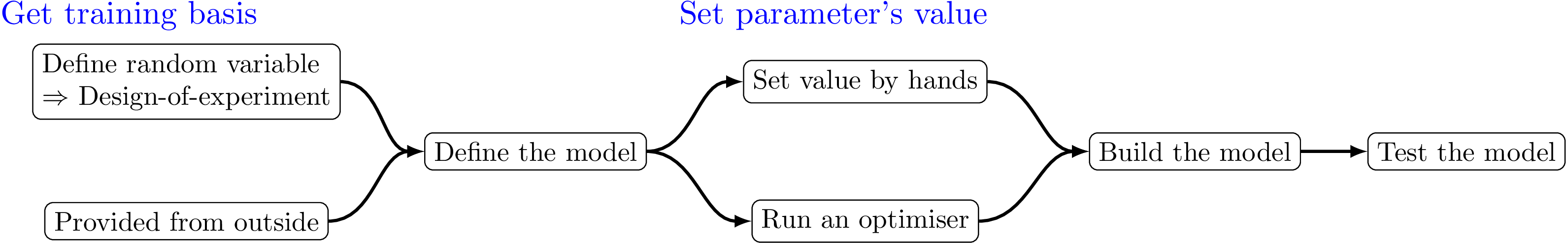
The kriging procedure in Uranie can be schematised in five steps, depicted in Figure IV.14. Here is a brief description of the steps:
get a training site. Either produced by a design-of-experiments from a model definition, or taken from anywhere else, it is mandatory to get this basis (the larger, the better).
set the parameter's values. It can be set by hands, but it is highly recommended to proceed through an optimisation, to get the best possible parameters.
build the kriging method.
test the obtained kriging model. This is done by running the kriging model over a new basis .
[8]
For  a gaussian vector, following the left-hand side relation below, meaning
that
a gaussian vector, following the left-hand side relation below, meaning
that  and
and
 are of
size
are of
size  and
and  and
and  are of size
 and the global covariance
matrix is made out of a
and the global covariance
matrix is made out of a  matrix of size
  , a
, a  matrix of size
  and a
and a  matrix of size
  defining also
  . Under the hypothesis that can be inverted, the law of conditionally to is gaussian and can be written as the right-hand side
equation below.
. Under the hypothesis that can be inverted, the law of conditionally to is gaussian and can be written as the right-hand side
equation below.

| |  | |
| IV.4. The artificial neural network |  | Chapter V. Sensitivity analysis |