

Documentation
/ Methodological guide
: 
| V.6. Fourier-based methods | ||
|---|---|---|
 | Chapter V. Sensitivity analysis |  |
The Fourier Amplitude Sensitivity Test (FAST) [MCRAE198215, SALTELLI1998445] is a
procedure that provides a way to estimate the expected value and variance of the output variable of a model, along
with the contribution of the input factors to this variance. An advantage of it, is that the evaluation of
sensitivity can be carried out independently for each factor using just a set of runs because all the terms in a
Fourier expansion are mutually orthogonal. The main idea behind this procedure is to transform the  -dimensional integration into a
single-dimension one, by using the transformation
-dimensional integration into a
single-dimension one, by using the transformation
where ideally,  is a set of angular frequencies said to be incommensurate (meaning that no frequency can be
obtained by linear combination of the other ones when using integer coefficients) and
is a set of angular frequencies said to be incommensurate (meaning that no frequency can be
obtained by linear combination of the other ones when using integer coefficients) and  is a transformation function chosen in order to ensure
that the variable is sampled accordingly with the probability density function of
is a transformation function chosen in order to ensure
that the variable is sampled accordingly with the probability density function of  (meaning that they are all uniformly distributed in their
respective volume definition). Given these conditions, the parametric variable
(meaning that they are all uniformly distributed in their
respective volume definition). Given these conditions, the parametric variable
 will evolve in
  and the vector
 traces out a curve that fills the entire -dimensional research volume. Practical considerations dictate that an integer
rather than an incommensurate set of frequencies must be used, with few consequences: the resulting parametric
curve is not longer a space-filling one, the fundamental of each input (the chosen frequency for this input) will
have harmonics that interfere with one another and the parametric curve becomes periodic with a
traces out a curve that fills the entire -dimensional research volume. Practical considerations dictate that an integer
rather than an incommensurate set of frequencies must be used, with few consequences: the resulting parametric
curve is not longer a space-filling one, the fundamental of each input (the chosen frequency for this input) will
have harmonics that interfere with one another and the parametric curve becomes periodic with a  -period.
When both and  are properly chosen, one can approximate the
following relations:
are properly chosen, one can approximate the
following relations:

where  and
and  and
and  are the Fourier coefficients, defined as

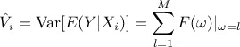
The first order coefficient is then obtained by estimating the variance for a fundamental and its harmonics. This can be done by using the second half of Equation V.6 running over
 instead of
  and replacing in the index by
  . The important point to
notice, for a real computation, is the limitation of the sum that, in the previous equation, runs up to infinity. A
truncation is done by imposing a cut-off with a factor
. The important point to
notice, for a real computation, is the limitation of the sum that, in the previous equation, runs up to infinity. A
truncation is done by imposing a cut-off with a factor  called the interference factor (whose default
value in Uranie is set to 6). Knowing that the exact same replacements can be done to
obtain the corresponding Fourier coefficients in Equation V.7, the contribution to the output
variance of a certain frequency, i.e. the first order sensitivity index, can be expressed as
Finally, the sample size
called the interference factor (whose default
value in Uranie is set to 6). Knowing that the exact same replacements can be done to
obtain the corresponding Fourier coefficients in Equation V.7, the contribution to the output
variance of a certain frequency, i.e. the first order sensitivity index, can be expressed as
Finally, the sample size  used to measure these coefficients should respect the
relation
used to measure these coefficients should respect the
relation  .
.
The Random Balance Design (RBD) [Tarantola2006717] method selects
design points over a curve
in the input space. The input space is explored here using the same frequency  . However the curve is not space-filling, therefore, we
take random permutations of the coordinates of such points, to generate a set of scrambled points that cover the
input space. The model is then evaluated at each design point. Subsequently, the model outputs are re-ordered such
that the design points are in increasing order with respect to factor . The Fourier spectrum is calculated on the model
output at the frequency and at its higher harmonics
. However the curve is not space-filling, therefore, we
take random permutations of the coordinates of such points, to generate a set of scrambled points that cover the
input space. The model is then evaluated at each design point. Subsequently, the model outputs are re-ordered such
that the design points are in increasing order with respect to factor . The Fourier spectrum is calculated on the model
output at the frequency and at its higher harmonics  and yields the estimate of the
sensitivity index of factor . The model outputs are re-ordered with respect to the other factors to obtain all the other
sensitivity indices.
and yields the estimate of the
sensitivity index of factor . The model outputs are re-ordered with respect to the other factors to obtain all the other
sensitivity indices.
In practice the RBD approach selected design points can be written as:

where  and
and  denotes the i-Th
random permutation of the
points. The values of the model output
denotes the i-Th
random permutation of the
points. The values of the model output  , for
, for  are computed and then are reordered (
 ) in order to get the corresponding values of
  ranked in increasing order. The
sensitivity of
ranked in increasing order. The
sensitivity of  to
is determined by the
harmonic content of
to
is determined by the
harmonic content of  , which
is quantified by its Fourier spectrum:
, which
is quantified by its Fourier spectrum:
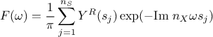
evaluated at equal to 1 and its higher harmonics (2, 3,..., up to
equal to 6 in our case),
leading to
This relation is used to estimate all the  , by re-ordering the output to
rank the i-Th input in an increasing order, which provides a complete estimation of the variance. Thanks
to the use of permutations, the total cost is of the order of assessments instead of the order of
, by re-ordering the output to
rank the i-Th input in an increasing order, which provides a complete estimation of the variance. Thanks
to the use of permutations, the total cost is of the order of assessments instead of the order of  for the FAST one.
In the implementation done within Uranie there are several modifiable parameters that can be considered before starting an analysis using the FAST method:
The transformation function
chosen among the following list:
Cukier:
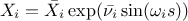
SaltelliA:

SaltelliB:

In this list,
 is the nominal value of the factor ,
  denotes the endpoints that define the estimated range of uncertainty of ,
  is a random phase shift taken value in
  and
evolves in
and
evolves in  .
.
The interference factor:
can be changed as well.
The frequencies: by providing a vector, it is possible to set a default at the frequencies' value used instead of having them determined by a specific algorithm to avoid, as best as possible, the interference.
The only common parameter changeable for both methods (and directly in the construction) is the number of samples.
| |  | |
| V.5. The Sobol method |  | V.7. The Johnson relative weight |