

Documentation
/ Methodological guide
: 
| Chapter VI. Dealing with optimisation issues | ||
|---|---|---|
 |  | |
Table of Contents
An optimisation is a complex problem, because each study has its own peculiarities and it often requires to grope one's way forward, before finding an interesting solution. Most commonly, when dealing with optimisation, there are:
one or more objectives that one wants to minimise (or maximise).
decision variables that have a clear influence on the objectives.
possibly some constraints either on the decision variables, on combination of some of them, or on objectives (defining the search domain)
Knowing this, it is also compulsory to choose an optimisation algorithm, which is a crucial part of the optimisation procedure. It is possible to divide these algorithms into two different categories:
local ones: they allow mono-criterion optimisation, with or without constraints. They are generally computationally efficient, but can not be used in parallel and tend to be trapped in local optima.
global ones: they allow multi-objective optimisation, with or without constraints. They are suitable for problems with many local optima, but are expensive computationally. However, they are easily parallelisable.
In the rest of this section, we will discuss optimisation procedure either in single-criterion or multi-objective
case. Independently of the chosen configuration the problem depends on input variables which will be gathered in a
vector  , called optimisation variable or decision variable. Each of
these variables can be constrained, i.e. following simple functions (as inequality) or more
complicated ones, that can be combination of several variables. The most obvious constraints are the boundaries: they
define the minimum and maximum values authorised for all the inputs, defining then the research
space.
, called optimisation variable or decision variable. Each of
these variables can be constrained, i.e. following simple functions (as inequality) or more
complicated ones, that can be combination of several variables. The most obvious constraints are the boundaries: they
define the minimum and maximum values authorised for all the inputs, defining then the research
space.
In the case of a single criterion problem, the optimisation procedure is equivalent to the minimisation of a function
 which is called the cost function (but also objective function depending on
the literature). The optimisation leads to the determination of a minimum (that can be called
optimum) that can either be global (there is no
which is called the cost function (but also objective function depending on
the literature). The optimisation leads to the determination of a minimum (that can be called
optimum) that can either be global (there is no  in the research volume such as
 ) or local (same relation as before, but only in the vicinity
of
) or local (same relation as before, but only in the vicinity
of  ).
).
As already discussed above, the optimisation is usually a minimisation problem of one or more objectives. We will discuss here the multi-objective case as it leads to the definition of the Pareto front and the Pareto set. The optimisation procedure can then be expressed as the minimisation of this function:

where  is the number of objectives imposed and
  is, here, the complete cost function. Unlike the
single-criterion case, there might be no such thing as an overall optimum since it is usually not possible to
quantify a relation between the objectives (to state which one is more important than the other). In the case where
two solutions (
is, here, the complete cost function. Unlike the
single-criterion case, there might be no such thing as an overall optimum since it is usually not possible to
quantify a relation between the objectives (to state which one is more important than the other). In the case where
two solutions ( and
and  ) are
possible, one can say that
dominates if the former does
as good as the latter for all the objectives but at least one, where it does better. The most common thing is to look
for a group of solutions that are said to be not dominated, meaning that they dominate the rest
of the solutions (that do not belong to this group) but each and every one of them can not dominate the
others. No-one can state whether one solution in this group is better than any other in the group (unless an external
constraint or preference is imposed, usually with hindsight). This definition goes along with the concept of trade
off. The group of not-dominated solutions is then called the Pareto set and its graphical
representation in the objective space is called the Pareto front. Finally, in the objective space,
one can represent the ideal point and Nadir point which are respectively
the minimum and maximum of all objective when considered separately in the Pareto front.
) are
possible, one can say that
dominates if the former does
as good as the latter for all the objectives but at least one, where it does better. The most common thing is to look
for a group of solutions that are said to be not dominated, meaning that they dominate the rest
of the solutions (that do not belong to this group) but each and every one of them can not dominate the
others. No-one can state whether one solution in this group is better than any other in the group (unless an external
constraint or preference is imposed, usually with hindsight). This definition goes along with the concept of trade
off. The group of not-dominated solutions is then called the Pareto set and its graphical
representation in the objective space is called the Pareto front. Finally, in the objective space,
one can represent the ideal point and Nadir point which are respectively
the minimum and maximum of all objective when considered separately in the Pareto front.
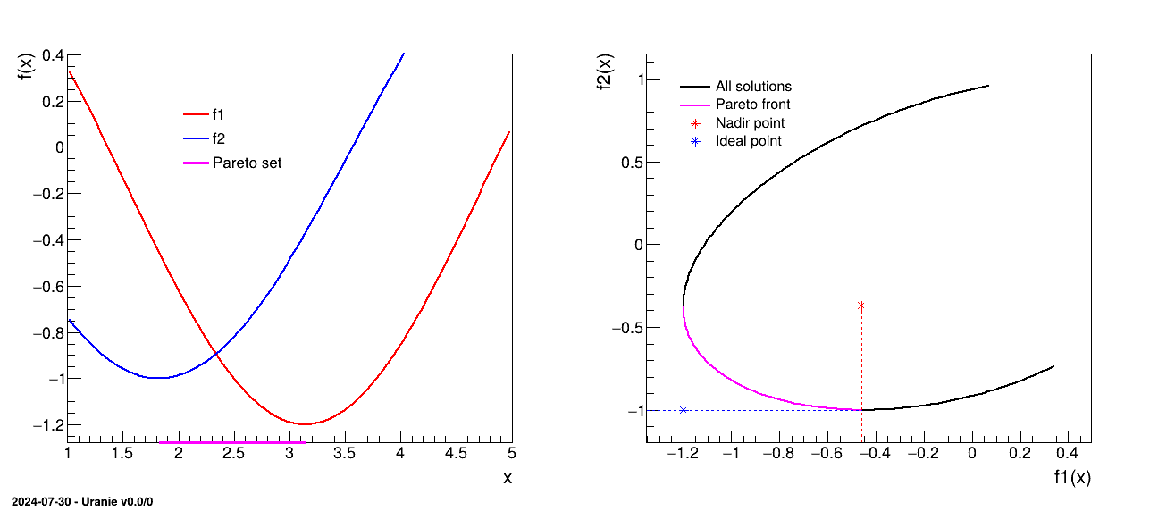
Figure VI.1 shows a very simple example of a pure analytic model with two objectives (the blue and red
curves on the left panel) depending only on one variable. In this simple case, the Pareto set is shown in pink, as
the area in between both criterion's minimum. Now looking in the criterion's space (right panel of Figure VI.1), all the solutions are shown in black and the corresponding Pareto front is, once more,
depicted in pink. Both the ideal and Nadir points are represented for illustration purpose.
Figure VI.1. Naive example of an imaginary optimisation case relying on two objectives that only depend on a single input variable.
 |
| | | |
| V.8. Sensitivity Indices based on HSIC |  | VI.2. Multicriteria optimisation |