

Documentation
/ Guide méthodologique
: 
| VI.2. Multicriteria optimisation | ||
|---|---|---|
 | Chapter VI. Dealing with optimisation issues |  |
A genetic algorithm is based on the way the genes are organised in a living being and the way they might evolve through time and through the future generations.
Genetic is the study of genes which are the places where all information concerning a being are encoded. These genes are gathered in some kind of containers named chromosomes. Depending on the being under consideration, the number of chromosomes will change (for instance, the human being has 23 types of chromosomes). In nature, the living beings can be split into two categories: those with only one chromosome per type (called haploid beings) and those with two chromosomes per type (called diploid beings). For the former, one precise characteristic is completely described by the corresponding gene in the chromosome. On the other hand, for the latter, the same characteristic is encoded by the two versions of the gene, called alleles, located on both chromosomes.
When considering a diploid being, another notion may arise: for every gene, it is possible to have twice the same allele or two different alleles on both chromosomes. When talking about this specific gene, the first case is called homozygote while the second is called heterozygote. The latter case will then leads to define the concept of dominance, whose existence is possible in two different forms: the true dominance when an investigated characteristic is only driven by the dominant allele, or the shared dominance when the resulting characteristic is an admixture of both alleles. In the former case, the characteristic will be defined by one allele (called the dominant one while the other is being called the recessive one).
Finally, evolution of the genotype through generations can come from two processes: the crossing one (when two beings are combining themselves to create a new one) and the mutation one (that happened spontaneously changing slightly one or several genes). The complete description of the genes in a being under study, is called genotype, while the complete description of its characteristics is called phenotype.
The genetic algorithm implemented in Uranie is a diploid algorithm with real-coding and true dominance. In other words, it means that every gene has two values (allele) which are represented by a double number, and the phenotype for this gene is driven either by one allele or the other (but not an admixture of both version). The implementation is done by plugging the Vizir package [Vizir] which is developed by Gilles Arnaud. The concept of homozygote or heterozygote (that should apply at the gene level) is applied here at the being level, implying that if a candidate is flagged as homozygote, it means that all genes on a certain chromosome are rigorously identical on the second one.
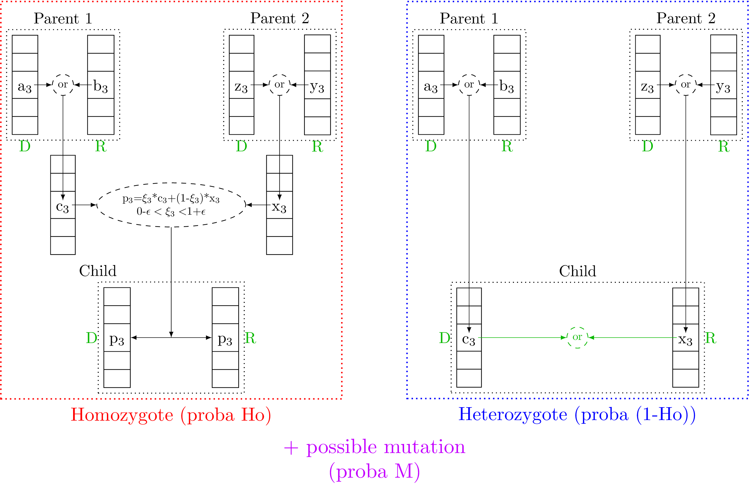
Concretely the implementation is done as follows: a chromosome is a fixed-size vector of double (the size being the number of gene, i.e. the number of criteria). At the initialisation, the value for the gene are chosen in the research space of the corresponding criteria, following a random drawing (like a SRS one). The next step, the pairing by two to create a candidate (as the considered beings are diploid), is complex and very much alike the crossing step to create children from selected candidates. Based on the Figure VI.2, this procedure is described below, split in several steps: starting from two parents (selected candidate of the N-Th generation) the crossing recipe to get N+1-Th generation candidate is
- Draw one chromosome per parent
In Uranie the chromosome is not taken as it is (copied) from the N-Th generation, but instead a new chromosome is created, taking randomly allele from the first or second chromosome of the corresponding parent. Once this is done twice, we obtain two chromosomes that should be associated to form a being. This step is present in Figure VI.2 both in the red and blue parts, whose difference is explained in the next step.
- Create homozygote being
In Uranie the concept of homozygote or heterozygote (that should apply to gene, c.f. Section VI.2.1.1) is applied to the considered being. There is a certain probability
 for the being to be
homozygote (the default value in Uranie being 50%). To do that, the two gathered chromosomes are scanned,
and for every genes a linear sum is done between both alleles using a real coefficient randomly drawn in
for the being to be
homozygote (the default value in Uranie being 50%). To do that, the two gathered chromosomes are scanned,
and for every genes a linear sum is done between both alleles using a real coefficient randomly drawn in
 (this
(this  can help a bit exploring the research space). The
results is stored in a new vector (chromosome) which is duplicated to get a new being with two identical
chromosome that we call an homozygote candidate (red part in Figure VI.2). On the contrary, if the zygote probability is in
can help a bit exploring the research space). The
results is stored in a new vector (chromosome) which is duplicated to get a new being with two identical
chromosome that we call an homozygote candidate (red part in Figure VI.2). On the contrary, if the zygote probability is in
 , the candidate will be called heterozygote (blue part in Figure VI.2).
- Determine the phenotype
The phenotype is determined by the dominant or recessive character of alleles, which is shown by the green part in Figure VI.2. The first and second steps discussed here to draw one chromosome per parent and create or not a homozygote being, do not take this information into account at all. The finalisation of the candidate consists then in doing a new random drawing for every gene, in order to determine which allele will be the dominant one. Once this is settled, the dominant one is put in the first vector (chromosome) of the candidate, for the sake of simplicity when testing the candidate. This is why in the parents and the resulting children, disregarding the candidate is homozygote and heterozygote, a capital D is found below the first chromosome (for dominant) while a capital R is written below the second one (for recessive).
- Mutate genes
To keep on exploring the research space, a random drawing is performed in order to know whether the resulting candidate should mutate. This step is also applied both to homozygote and heterozygote candidate, with a probability
 whose default
value in Uranie is 1%. If selected, a gene is chosen in both chromosomes of the candidate (not necessarily
the same gene, as this choice is as well coming from random drawing) and a new randomly-drawn value is stored
instead of the one already there.
whose default
value in Uranie is 1%. If selected, a gene is chosen in both chromosomes of the candidate (not necessarily
the same gene, as this choice is as well coming from random drawing) and a new randomly-drawn value is stored
instead of the one already there.
- Test and validate the children
The newly produced candidates are then tested.
Figure VI.2. Description of the children production process in the Uranie implementation of the genetic algorithm
 |
This section introduces the discussion from [ManyObj] which is a CEA technical note. The idea is to provide access to dedicated references and provide the vocabulary, if the reader cannot either access the catalog of CEA notes or read french (otherwise Ref. [ManyObj] is the one to consult, the rest of this section can be discarded).
Unlike classical optimisation algorithm whose research is basically sequential from a given starting point, an evolutionary algorithm starts from a random sample (a population) which evolves thanks to:
selection operators: how to choose the parents, i.e. the best element that should be the starting point to new elements (parental selection) and how to remove the less interesting one (environmental selection).
variation operators: how to produce a new elements from existing ones (crossing), how to randomly alterate some caracters (mutation) and how to correct some caracters to make a new element viable (reparation, optional one).
When dealing with multi-objective problems, the notion of Pareto set and front is quickly arising as one wants to obtain a pareto set, i.e. an ensemble of non-dominated solutions. The solutions should ideally obey different properties:
convergence: be as close as possible to the "real" pareto front usually called the Pareto-optimal front;
coverage: coverage the widest range possible;
density: elements of the set should be reparted as evenly as possible on the obtained coverage.
Discussions about these notions can be found for instance in [zitzler2010set] and in [zitzler1999evolutionary].
Is is simple to spot that 2 things can separatly bring a poor convergence of a finite pareto set:
the size of the requested population;
the number of objectives to be minimised.
If the only criteria to stop an evolutionary algorithm is the fact that the ensemble of solution are non-dominated one to another, then clearly having a large number of criteria will lead to have non-comparable solutions almost out-of-box (at the initialisation level). Even with only two criteria, but a small number of requested element in the final population, putting the solution away one to another to improve the coverage will automatically reduce the convergence as the competition between elements will diminish. Even the crossing could become problematic: given a very large Pareto front, crossing very different elements might lead far away new resulting elements, meaning an inefficiency in the generation steps.
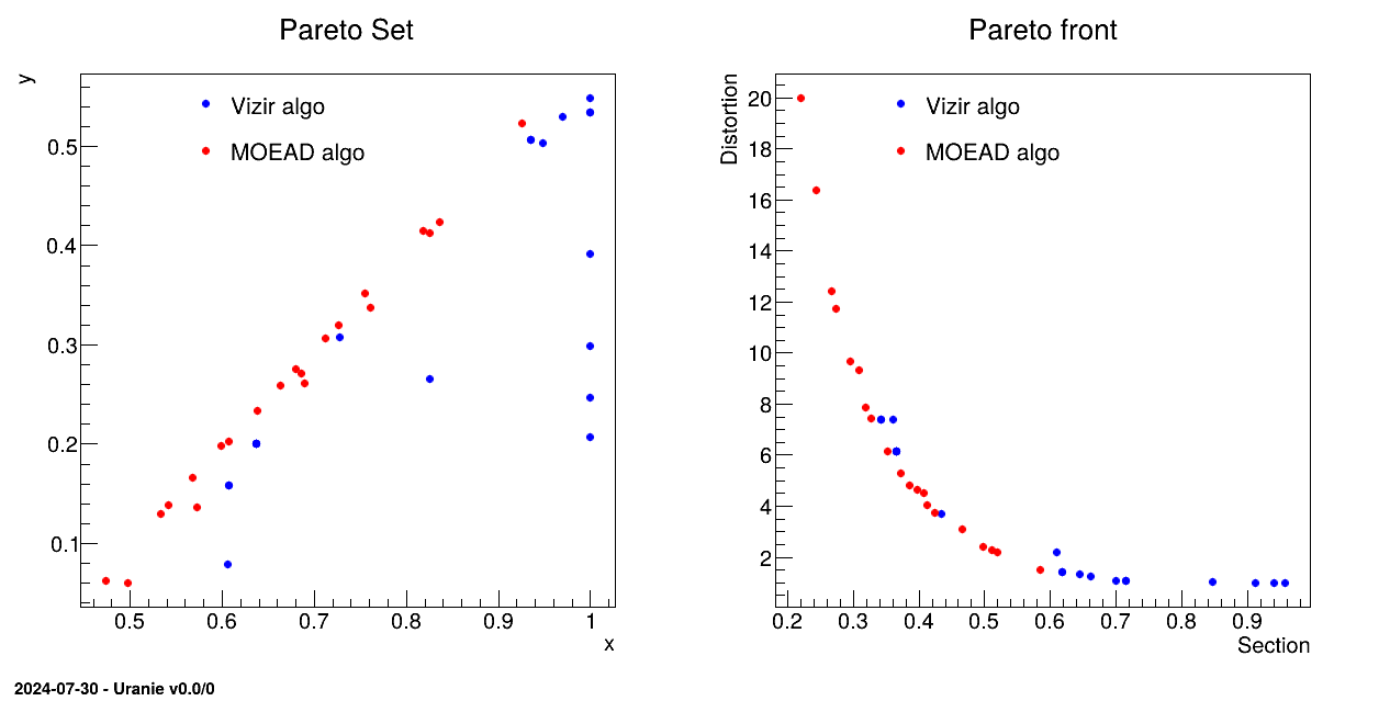
Figure VI.3 shows a dummy example of this, using our classical hollow bar example introduce in the user manual, asking only 20 elements in the final population. The classical genetic algorithm (blue dots) stops with the non-dominance criteria, so to obtain this only 100 estimations are needed in total. If one compares the way the solutions are distributed in the criteria space (the Pareto Front), the coverage, density and convergence are worse than the curve shown by the red dots. These dots are the 20 solutions proposed by the MOEAD implentation (see next section below) that decomposes the space before starting the initialisation and is not only relying on dominance to perform the different operation stated above.
Figure VI.3. Comparison of two Pareto sets (left) and fronts (right) from vizir (blue) and MOEAD (ref) when the hollow bar case is studied with very low number of points, i.e. about 20 (simulating higher dimensions).
 |
This section provides a simple list of algorithms and their references, that can deal with many-objective optimisation. They have been splitted in different categories, among which
those who rely on distance or isolation notion to sort out solution which have the same rank (once pareto-dominance ranking is done);
those who try to generalise pareto ranking to make it more discriminant;
those who no longer use pareto rank but try to set up quality index instead;
those who split the domain first, in order to get a better coverage at first of the ensemble of solutions.
In Uranie one would find different implementation of many-objective algorithms that enrich the possibility and capacity of the usual evolutionary algorithm, among which:
a knee-point one [zhang2015knee]
an IBEA one (Indicator Based Evolutionary Algorithm) [zitzler2004indicator]
an MOEAD one (Multi Objective Evolutionary Algorithm based on Decomposition) [zhang2007moea]
| |  | |
| Chapter VI. Dealing with optimisation issues |  | Chapter VII. The Calibration module |