Documentation / Methodological guide :

This method consists mainly of the analytical formulation of the posterior distribution under assumptions: the problem can be considered linear and the prior distributions are normally distributed (or non-informative/flat, as noted at the end of this section).

In the specific case of a linear model, one can then write where is the regressor vector. This way of writing the model can include an "hidden virtual" whose purpose is to integrate a constant term into the regression (to describe a pedestal). Using the statistical approach introduced in Section VII.1, one can also define the covariance matrix of the residuals which will be written hereafter as

From there, one can construct the design matrix whose columns define the subspace onto which the model is projected. With a normal prior, which follows the form the posterior is also expected to be normal, so it can be written 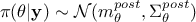where its parameters are expressed as

Equation VII.7. 

and

Equation VII.8. 

It is also possible, as introduced in Section VII.1.2.3, to use a non-informative prior such as Jeffrey's prior: it is an improper flat prior () [bioche2015approximation], whose posterior distribution (in the linear case) is also Gaussian. For this prior, the posterior parameters are equivalent to those obtained with a Gaussian prior, given in Equation VII.7 and Equation VII.8 with all references to removed:

Equation VII.9. 

This final form corresponds to the expected results obtained when only considering linear regression within the weighted least squares approach [Fry2010].

VII.3.1. Prediction values

Once both the posterior parameter values and covariances are estimated, it is possible to make a prediction for a dataset not used in the estimation. The central value of the prediction is easy to get, as with any other methods presented in this documentation, since one knows the model and can use the newly estimated posterior mean values of the parameters.

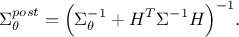
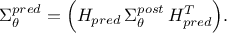
The novel aspect is that a variance can also be estimated for the predicted mean using the posterior covariance matrix of the parameters, , already introduced in Equation VII.8. This variance represents the uncertainty in each new predicted point due to parameter uncertainty, and it is contained in the covariance matrix of dimension , where is the sample size under consideration. To obtain the estimate, one needs the new design matrix which then leads to

Equation VII.10.