

Documentation
/ Guide méthodologique
: 
| VII.4. Approximate Bayesian Computation techniques (ABC) | ||
|---|---|---|
 | Chapter VII. The Calibration module |  |
This section covers methods grouped under the acronym ABC, which stands for Approximate Bayesian Computation. The core idea is to perform Bayesian inference without explicitly evaluating the model likelihood function. For this reason, these methods are also refered to as likelihood-free algorithms [wilkinson2013approximate].
As a reminder, the principle of the Bayesian approach is summarized in the equation
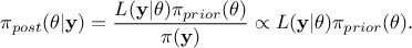 , where
  is the conditional probability of the observations given the parameter values
  ,
,  is the a
priori probability density of (the prior), and
is the a
priori probability density of (the prior), and  is the marginal likelihood of the observations, which is constant.
It does not depend on the values of but only on its prior, as
is the marginal likelihood of the observations, which is constant.
It does not depend on the values of but only on its prior, as  making it a normalizing factor. For more details, see
Section VII.1.2.3.
making it a normalizing factor. For more details, see
Section VII.1.2.3.
Rejection ABC is the simplest version of the ABC approach. Its origins date back to the 1980s
[rubin1984bayesianly] and it is possible to see a nice introduction of the rejection algorithm
as originally applied to a problem with a finite countable set  of values in [marin2012approximate]. In
this specific case, it only consisted in two random draws: the parameter values according to their prior then the
model prediction according to the parameter values just drawn. If the result was an element of the reference
dataset, the configuration was kept.
of values in [marin2012approximate]. In
this specific case, it only consisted in two random draws: the parameter values according to their prior then the
model prediction according to the parameter values just drawn. If the result was an element of the reference
dataset, the configuration was kept.
Things become more complicated when considering continuous sample spaces, since there is no such thing as strict equality when considering stochastic behaviour (without even discussing the numerical issues that have to arise at some points). This implies the need for two important concepts
a distance metric in the output space, denoted
 ;
;
a tolerance parameter, denoted
 ,
which determines the accuracy of the algorithm.
,
which determines the accuracy of the algorithm.
Unlike the simpler discrete case quickly introduced above where the aim is to have strict equality between the predictions and the reference data, here the accepted configurations would be those fulfilling the following condition

where  is the configuration under study drawn
from the prior
is the configuration under study drawn
from the prior  and
and  is the model predictions generated from
  once run on the reference dataset. This was firstly used in the
late nineties, as can be seen in [pritchard1999population].
once run on the reference dataset. This was firstly used in the
late nineties, as can be seen in [pritchard1999population].
Warning
One should recall that the uncertainty model is defined on the residuals, as stated in Equation VII.1 and that residuals are usually considered normally distributed, as in Equation VII.2. Disregarding the origin of these residuals, as discussed in Section VII.1, if the model one is providing is deterministic, the calibration will focus on a single realisation of the observation without uncertainty consideration. In this case, the model prediction must be modified to include a noise representative of the residuals hypotheses [van2018taking].
This methodology shows that accepted configurations are not directly sampled from the true posterior distribution
 but rather come from an approximation of it that can be written
 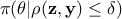 . Two interesting asymptotic regimes can be highlighted:
when
 : the algorithm is exact and converges to the true posterior ;
when
 : the algorithm ignores the reference data and simply returns the original prior
.
: the algorithm ignores the reference data and simply returns the original prior
.
There are many different versions of this kind of algorithm, among which one could find an extra step using summary
statistics  to project
both and
to project
both and
 onto a lower
dimensional space. In this version, the configurations kept are drawn from
onto a lower
dimensional space. In this version, the configurations kept are drawn from 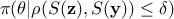 .
.
Finally, another possible way to select the best representative sub-sample might be by using a percentile of the analysed
and computed set of configurations. Although, mainly recommended for high-dimensional cases (i.e., when
 becomes large), this
solution might work as long as one keeps an eye on the residuals distribution provided by the a posteriori
estimated parameters. Indeed, if no threshold is chosen but a percentile is used, the requested number of configurations
will always be obtained in the end, but the only way to check whether the uncertainty assumptions are valid is to assess
how closely the predictions match the full reference dataset.
becomes large), this
solution might work as long as one keeps an eye on the residuals distribution provided by the a posteriori
estimated parameters. Indeed, if no threshold is chosen but a percentile is used, the requested number of configurations
will always be obtained in the end, but the only way to check whether the uncertainty assumptions are valid is to assess
how closely the predictions match the full reference dataset.
| |  | |
| VII.3. Analytical linear Bayesian estimation |  | VII.5. Markov chain Monte Carlo approach |