Documentation / User's manual in C++ :

III.2. The Stochastic methods

III.2. The Stochastic methods
	Chapter III. The Sampler module

III.2. The Stochastic methods

III.2.1. Introduction

The stochastic classes all inherit from the TSampler class through the TSamplerStochastic one. In these classes the knowledge (or mis-knowledge) of the model is encoded in the choice of probability law used to describe the inputs , for . These laws are usually defined by:

a range that describes the possible values of
the nature of the law, which has to be taken in the list of TStochasticAttribute already presented in Section II.2.5

A choice has frequently to be made between two implemented methods of drawing:

SRS (Simple Random Sampling):: This method consists in independently generating the samples for each parameter following its own probability density function. The obtained parameter variance is rather high, meaning that the precision of the estimation is poor leading to a need for many repetitions in order to reach a satisfactory precision. An example of this sampling when having two independent random variables (uniform and normal one) is shown in Figure III.3-left.
LHS (Latin Hypercube Sampling):: this method [McKay2000] consists in partitioning the interval of each parameter so as to obtain segments of equal probabilities, and afterwards in selecting, for each segment, a value representing this segment. An example of this sampling when having two independent random variables (uniform and normal one) is shown in Figure III.3-right.

Both methods consist in generating a -sample represented by a matrix called matrix of the design-of-experiments. The number of columns of the matrix correspond to the number of uncertain parameters , and the number of lines is equal to the size of the sample .

The first method is fine when the computation time of a simulation is "satisfactory". As a matter of fact, it has the advantage of being easy to implement and to explain; and it produces estimators with good properties not only for the mean value but also for the variance. Naturally, it is necessary to be careful in the sense to be given to the term "satisfactory". If the objective is to obtain quantiles for extreme probability values (i.e. = 0.99999 for instance), even for a very low computation time, the size of the sample would be too large for this method to be used. When a computation time becomes important, the LHS sampling method is preferable to get robust results even with small-size samples (i.e. = 50 to 200) [Helton02]. On the other hand, it is rather trivial to double the size of an existing SRS sampling, as no extra caution has to be taken apart from the random seed.

In Figure III.2, we present two samples of size = 8 coming from these two sampling methods for two random variables according to a gaussian law, and a uniform law. To make the comparison easier, we have represented on both figures the partition grid of equiprobable segments of the LHS method, keeping in mind that it is not used by the SRS method. These figures clearly show that for LHS method each variable is represented on the whole domain of variation, which is not the case for the SRS method. This latter gives samples that are concentrated around the mean vector; the extremes of distribution being, by definition, rare.

Concerning the LHS method (right figure), once a point has been chosen in a segment of the first variable , no other point of this segment will be picked up later, which is hinted by the vertical red bar. It is the same thing for all other variables, and this process is repeated until the points are obtained. This elementary principle will ensure that the domain of variation of each variable is totally covered in a homogeneous way. 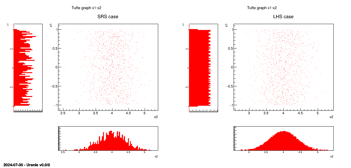On the other hand, it is absolutely not possible to remove or add points to a LHS sampling without having to regenerate it completely. A more realistic picture is draw in Figure III.3 with the same laws, both for SRS on the left and LHS on the right. The "tufte" representation (presented in Section II.5.6) clearly shows the difference between both methods when considering one-dimensional distribution.

Figure III.2. Comparison of the two sampling methods SRS (left) and LHS (right) with samples of size 8.

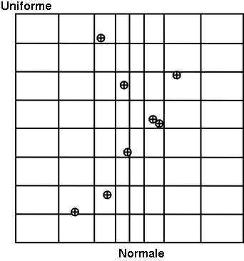
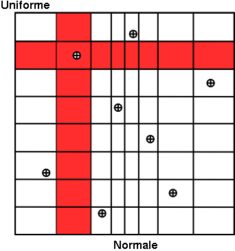
Figure III.3. Comparison of deterministic design-of-experiments obtained using either SRS (left) or LHS (right) algorithm, when having two independent random variables (uniform and normal one)

Comparison of deterministic design-of-experiments obtained using either SRS (left) or LHS (right) algorithm, when having two independent random variables (uniform and normal one)

There are two different sub-categories of LHS design-of-experiments discussed here and whose goal might slightly differs from the main LHS design discussed above:

the maximin LHS: this category is the result of an optimisation whose purpose is to maximise the minimal distance between any sets of two locations. This is discussed later-on in Section III.2.2.
the constrained LHS: this category is defined by the fact that someone wants to have a design-of-experiments fulfilling all properties of a Latin Hypercube Design but adding one or more constraints on the input space definition (generally inducing correlation between varibles). This is also further discussed in Section III.2.2 and in Section III.2.4.

Once the nature of the law is chosen, along with a variation range, for all inputs , the correlation between these variables has to be taken into account. This is further discussed in Section III.3

III.2.2. The main sampler classes

The sampler classes are built with the same skeleton. They consist in a three steps procedure: init, generateSample and terminate. There are five different types of Stochastic sampler that can be used:

TSampling: general sampler where the sampling is done with the Iman and Conover methods ([Iman82]) that uses a double Cholesky decomposition in order to respect the requested correlation matrix. This methods has the drawback of asking a number of samples at least twice as large as the number of attribute.
TBasicSampling: very simple implementation of the random sampling that can, as well, produce stratified sampling. As it is fairly simple, there is no lower limit in the number of random samples that can be generated and generation is much faster when dealing with a large number of attributes than with the TSampling. On the other hand, even though a correlation can be imposed between the variables, it will be done in a simple way that cannot by construction respect the stratified aspect (if requested, see [metho] explanations).
TMaxiMinLHS: class recently introduced to produced maximin LHS, whose purpose is to get the best coverage of the input space (for a deeper discussion on the motivation, see [metho]). It can be used with a provided LHS drawing or it can start from scratch (using the TSampling class to get the starting point). The result of this procedure can be seen in Figure XIV.13 which was procuded with the macro introduced in Section XIV.3.11;
Tip
The optimisation to get a maximin LHS is done on the mindist criterion: let 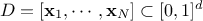be a design-of-experiments with points. The mindist criterion is written as: where is the euclidian norm.
This information can be computed on any grid, by calling the static function
```
double mindist = TMaxiMinLHS::getMinDist(TMatrixD LHSgrid);
```
TConstrLHS: class recently introduced to produced constrained LHS, whose purpose is to get nicely covered marginal laws while respecting one or more constraints imposed by the user. It can be used with a provided LHS drawing or it can start from scratch (using the TSampling class to get the starting point) and it is discussed a bit further in Section III.2.4. The result of this procedure can be seen in Figure XIV.14 which was procuded with the macro introduced in Section XIV.3.12;
TGaussianSampling: very basic sampler specially done for cases composed with only normal distributions. It relies on the drawing of a sample being the number of sample and the number of inputs. The sample is transformed to account for correlation (see [metho]) and shifted by the requested mean (for every variables).
TImportanceSampling: use the same method as TSampling but should be used when one TAttribute has a son. In this case the range for the considered attribute is the sub-range used to define the son and there is specific reweighting procedure to take into account the fact that the authorised range is reduced. LHS is therefore used by default.

III.2.3. Simple example

The following piece shows how to generate a sample using the TSampling class.

TUniformDistribution *xunif = new TUniformDistribution("x1", 3., 4.);     
TNormalDistribution  *xnorm = new TNormalDistribution("x2", 0.5, 1.5);    

TDataServer * tds = new TDataServer("tdsSampling", "Demonstration Sampling");
tds->addAttribute(xunif);
tds->addAttribute(xnorm);

// Generate the sampling from the TDataServer object
TSampling *sampling = new TSampling(tds, "lhs", 1000); 
sampling->generateSample(); 
tds->drawTufte("x2:x1");

Generation of a design-of-experiments with stochastic attributes

	Generating a uniform random variable in [3., 4.]
	Generating a gaussian random variable with a mean of 0.5 and a standard deviation of 1.5
	Construct the sampler object requesting a sample of 1000 events, using the Lhs algorithm.
	Method to generate the sample.
	Draw the plot as the right side of Figure III.3

III.2.4. TConstrLHS example

This section will discuss the way to produce a constrained LHS design-of-experiments from scratch, focusing on the main problematic part: defining one or more constraints and on which variable to apply them. The logic behind the heuristic is supposed to be known, so if it's not the case, please have a look at the dedicated section in [metho]. This section will mostly rely on the way to define the constraints and the variables on which these should be applied on which are specified by the method addConstraint. This methods takes 4 arguments:

a pointer to the function that will compute the constraints values;
the number of constraint defined in the function discussed above;
the number of parameters that are provided to the function discussed above;
the values of the parameters that are provided to the function discussed above;

The main object is indeed the constraint function and the way it is defined is discussed here. It is a C++ function (for convenience as the platform is C++-coded) but this should not be an issue even for python users. The followings lines are showing the example of the constraint function used to produce the plot in Section XIV.3.12.


void Linear(double *p, double *y)
{
    double p1=p[0], p2=p[1];
    double p3=p[2], p4=p[3];

    // Linear constaint
    y[0] = (( (p1 + p2>=2.5) || (p1-p2<=0) ) ? 0 : 1);
    y[1] = ((p3 - p4<0) ? 0 : 1);

}

Here are few elements to discuss and explain this function:

its prototype is the usual C++-ROOT one with a pointer to the input parameter p and a pointer to the output (here the constraint results) y;
the first lines are defining the parameters, meaning the couples for all the constraints. By convention, the first element of every line ( and ) are of the row type (they will not change in the design-of-experiments through this constraint, see [metho] for clarification) while the second parameters ( and ) are of the column type, meaning their order in the design-of-experiments will change through permutations through this constraint.
the rest of the lines are showing the way to compute the constraints and to interpret them thanks to the trilinear operator (even though the classical if, else would perfectly do the trick as well. Let's focus first on the second constraint:
```
y[1] = ((p3 - p4<0) ? 0 : 1);  
```
if p3 is lower than p4 (p3-p4<0) then the function will put 0 in y[1] (stating that this configuration is not fulfilling the constraint), and it will put 1 otherwise (stating that the constraint is fulfilled). The other line is defining another constraint which is composed of two tests on the same couple of variables:
```
y[0] = (( (p1 + p2>=2.5) || (p1-p2<=0) ) ? 0 : 1); 
```
Here, two constraints are combined in once, as they affect the same couple of variables, the configuration will be rejected either if p1+p2 is greater than 2.5 or if p1 is lower than p2.

Once done, this function needs to be plugged into our code in order to state what variables are p1, p2, p3 and p4 so that the rest of the procedure discussed in [metho] can be run. This is done in the addConstraint method, thanks to the third and fourth paramaters which are taken from a single object: a vector<int> in C++ and a numpy.array in python. It defines a list of indices (integers) that corresponds to the number of the input attributes as it is has been added into the TDataServer object. For instance in our case, the list of input attributes is "x0:x1:x2" while the constraints are coupling and respectively. Once translated in term of indices, the constraints are coupling respectively and , so the list of parameter should reflect this which is shown below:

vector<int> inputs = {1,0,2,1};
constrlhs->addConstraint(Linear, 2, inputs.size(), &inputs[0]);

Warning

The consistency between the function and the list of parameters is up to you and you should keep a carefull watch over it. It is true that an inequality can be written in two ways, as

but when the constraint is defined as

y[0] = ((p[0] - p[1]<0) ? 0 : 1);

the results will be drastically different if the list of parameters is

(which should fulfill the constraint shown above) or

which would results in the exact opposite behaviour (and might make the heuristic crash if the constraint cannot be fulfilled).


Chapter III. The Sampler module		III.3. Description of a correlation