Documentation / User's manual in C++ :

The objective of the macro is to build a multilinear regression between the predictors related to the normalisation of the variables x1, x2, x3, x4, x5, x6, x7 and a target variable y from the database contained in the ASCII file cornell.dat:

#NAME: cornell
#TITLE: Dataset Cornell 1990
#COLUMN_NAMES: x1 | x2 | x3 | x4 | x5 | x6 | x7 | y
#COLUMN_TITLES: x_{1} | x_{2} | x_{3} | x_{4} | x_{5} | x_{6} | x_{7} | y

0.00 0.23 0.00 0.00 0.00 0.74 0.03 98.7
0.00 0.10 0.00 0.00 0.12 0.74 0.04 97.8
0.00 0.00 0.00 0.10 0.12 0.74 0.04 96.6
0.00 0.49 0.00 0.00 0.12 0.37 0.02 92.0
0.00 0.00 0.00 0.62 0.12 0.18 0.08 86.6
0.00 0.62 0.00 0.00 0.00 0.37 0.01 91.2
0.17 0.27 0.10 0.38 0.00 0.00 0.08 81.9
0.17 0.19 0.10 0.38 0.02 0.06 0.08 83.1
0.17 0.21 0.10 0.38 0.00 0.06 0.08 82.4
0.17 0.15 0.10 0.38 0.02 0.10 0.08 83.2
0.21 0.36 0.12 0.25 0.00 0.00 0.06 81.4
0.00 0.00 0.00 0.55 0.00 0.37 0.08 88.1

{
  TDataServer * tds = new TDataServer();
  tds->fileDataRead("cornell.dat");
  
  tds->normalize("*", "cr");  // ("x1:x2:x3:x4:x5:x6:y", "cr", TDataServer::kCR)
  
  TCanvas *c = new TCanvas("c1", "Graph for the Macro modeler",5,64,1270,667);
  TPad *pad = new TPad("pad","pad",0, 0.03, 1, 1); pad->Draw();
  pad->Divide(2);
  pad->cd(1);
  tds->draw("y:x7");
  
  TLinearRegression *tlin = new TLinearRegression(tds,"x1cr:x2cr:x3cr:x4cr:x5cr:x6cr", "ycr", "nointercept");
  tlin->estimate();  
  
 pad->cd(2);
 tds->draw("ycr:ycrhat");
    
}

The ASCII data file cornell.dat is loaded in the TDataServer:

TDataServer * tds = new TDataServer();
tds->fileDataRead("cornell.dat");

The variables are all normalised with a standardised method. The normalised attributes are created with the cr extension:

tds->normalize("*", "cr");

The linear regression is initialised and characteristic values are computed for each normalised variable with the estimate method. The regression is built with no intercept:

TLinearRegression *tlin = new TLinearRegression(tds,"x1cr:x2cr:x3cr:x4cr:x5cr:x6cr", "ycr", "nointercept");
tlin->estimate();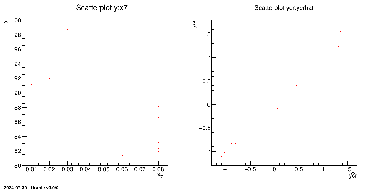

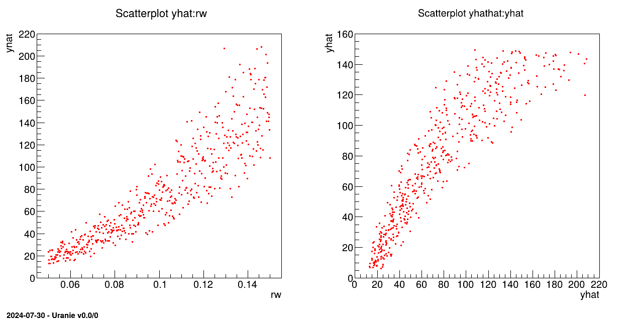
The objective of this macro is to build a linear regression between a predictor rw and a target variable yhat from the database contained in the ASCII file flowrate_sampler_launcher_500.dat defining values for the eight variables described in Section IV.1.2.1 on 500 patterns.

{
  TDataServer * tds = new TDataServer();
  tds->fileDataRead("flowrate_sampler_launcher_500.dat");
  
  TCanvas *c = new TCanvas("c1", "Graph for the Macro modeler",5,64,1270,667);
  TPad *pad = new TPad("pad","pad",0, 0.03, 1, 1); pad->Draw();
  pad->Divide(2);
  pad->cd(1); tds->draw("yhat:rw");
  
  //   tds->getAttribute("yhat")->setOutput();
  
  TLinearRegression *tlin = new TLinearRegression(tds, "rw","yhat");
  tlin->estimate();
 
  pad->cd(2); tds->draw("yhathat:yhat");
     
  tds->startViewer();
  
}

The TDataServer is loaded with the database contained in the file flowrate_sampler_launcher_500.dat with the fileDataRead method:

TDataServer * tds = new TDataServer();
tds->fileDataRead("flowrate_sampler_launcher_500.dat");

The linear regression is initialised and characteristic values are computed for rw with the estimate method:

TLinearRegression *tlin = new TLinearRegression(tds, "rw","yhat");
tlin->estimate();

The objective of the macro is to build a multilinear regression between the predictors , , , , , , , and a target variable yhat from the database contained in the ASCII file flowrate_sampler_launcher_500.dat defining values for these eight variables described in Section IV.1.2.1 on 500 patterns. Parameters of the regression are then exported in a .C file _FileContainingFunction_.C:

void MultiLinearFunction(double *param, double *res)
{
  ////////////////////////////// 
  //
  //     *********************************************
  //     ** Uranie v3.12/0 -  Date : Thu Jan 04, 2018
  //     ** Export Modeler : Modeler[LinearRegression]Tds[tdsFlowrate]Predictor[rw:r:tu:tl:hu:hl:l:kw]Target[yhat]
  //     ** Date : Tue Jan  9 12:08:27 2018

  //     *********************************************
  //
  //     *********************************************
  //     ** TDataServer 
  //     **        Name  : tdsFlowrate
  //     **        Title : Design of experiments for Flowrate
  //     **     Patterns : 500
  //     **   Attributes : 10
  //     *********************************************
  //
  //     INPUT  : 8
  //             rw : Min[0.050069828419999997] Max[0.14991758599999999] Unit[]
  //             r : Min[147.90551809999999] Max[49906.309529999999] Unit[]
  //             tu : Min[63163.702980000002] Max[115568.17200000001] Unit[]
  //             tl : Min[63.169232649999998] Max[115.90147020000001] Unit[]
  //             hu : Min[990.00977509999996] Max[1109.786159] Unit[]
  //             hl : Min[700.14498509999999] Max[819.81105760000003] Unit[]
  //             l : Min[1120.3428429999999] Max[1679.3424649999999] Unit[]
  //             kw : Min[9857.3689890000005] Max[12044.00546] Unit[]
  //
  //     OUTPUT : 1
  //             yhat : Min[13.09821] Max[208.25110000000001] Unit[]
  //
  ////////////////////////////// 
  //
  //     QUALITY  : 
  //
  //              R2  = 0.948985
  //              R2a = 0.948154
  //              Q2  = 0.946835
  //
  ////////////////////////////// 

  // Intercept
  double y = -156.03;

  // Attribute : rw
  y += param[0]*1422.21;

  // Attribute : r
  y += param[1]*-3.07412e-07;

  // Attribute : tu
  y += param[2]*2.15208e-06;

  // Attribute : tl
  y += param[3]*-0.00498512;

  // Attribute : hu
  y += param[4]*0.261104;

  // Attribute : hl
  y += param[5]*-0.254419;

  // Attribute : l
  y += param[6]*-0.0557145;

  // Attribute : kw
  y += param[7]*0.00813552;

  // Return the value
  res[0] = y;
}

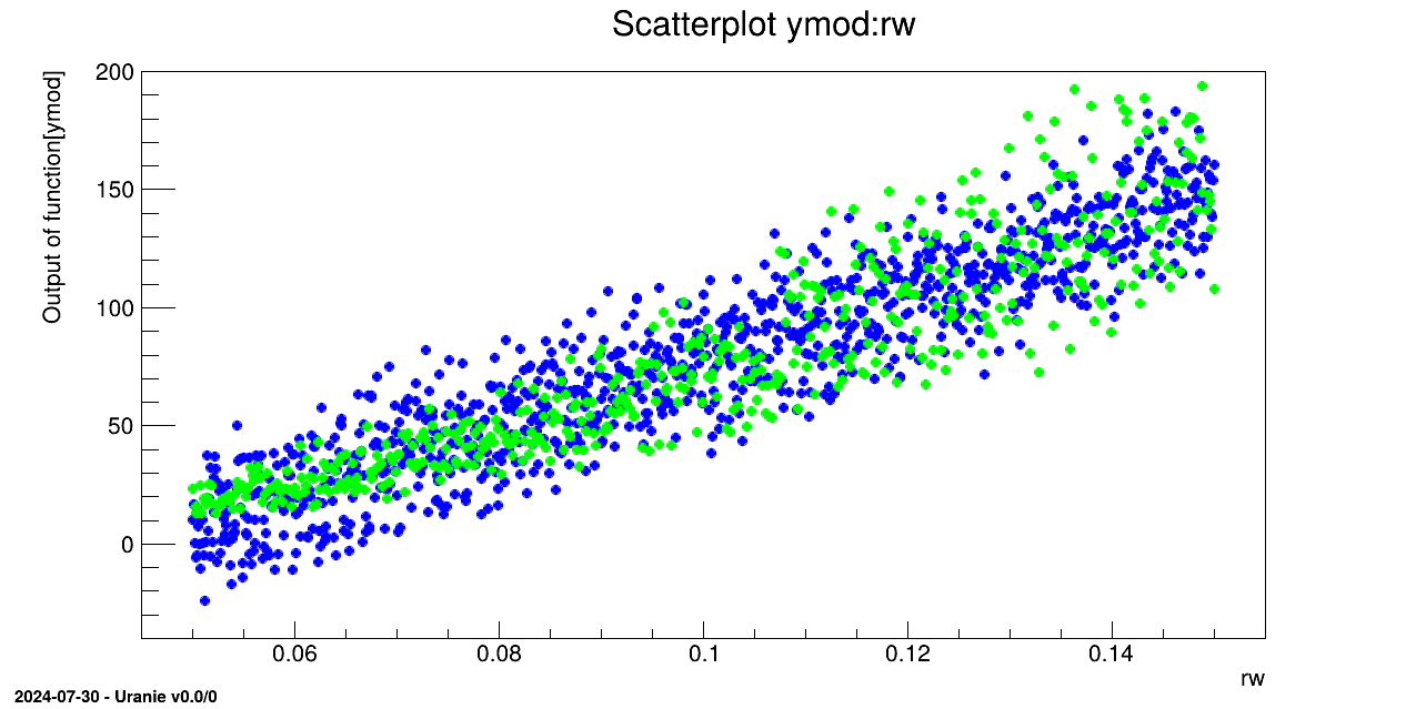
This file contains a MultiLinearFunction function. Comparison is made with a database generated from random variables obeying uniform laws and output variable calculated with this database and the MultiLinearFunction function.

{
  TDataServer * tds = new TDataServer();
  tds->fileDataRead("flowrate_sampler_launcher_500.dat");
  
  TCanvas *c = new TCanvas("c1", "Graph for the Macro modeler",5,64,1270,667);
  c->Divide(2);
  c->cd(1); tds->draw("yhat:rw");

  // tds->getAttribute("yhat")->setOutput();
  
  TLinearRegression *tlin = new TLinearRegression(tds, "rw:r:tu:tl:hu:hl:l:kw", "yhat");
  tlin->estimate();  
    
  tlin->exportFunction("c++", "_FileContainingFunction_", "MultiLinearFunction");

  // Define the DataServer
  TDataServer *tds2 = new TDataServer("tdsFlowrate", "Design of experiments for Flowrate");

  // Add the study attributes 
  tds2->addAttribute( new TUniformDistribution("rw", 0.05, 0.15));
  tds2->addAttribute( new TUniformDistribution("r", 100.0, 50000.0));
  tds2->addAttribute( new TUniformDistribution("tu", 63070.0, 115600.0));
  tds2->addAttribute( new TUniformDistribution("tl", 63.1, 116.0));
  tds2->addAttribute( new TUniformDistribution("hu", 990.0, 1110.0));
  tds2->addAttribute( new TUniformDistribution("hl", 700.0, 820.0));
  tds2->addAttribute( new TUniformDistribution("l", 1120.0, 1680.0));
  tds2->addAttribute( new TUniformDistribution("kw", 9855.0, 12045.0));

  Int_t nS = 1000;
  //   \test Générateur de plan d'expérience
  TSampling *sampling = new TSampling(tds2, "lhs", nS);
  sampling->generateSample();   
     
  gROOT->LoadMacro("_FileContainingFunction_.C");
  
  // Create a TLauncherFunction from a TDataServer and an analytical function
  // Rename the outpout attribute "ymod"
  TLauncherFunction * tlf = new TLauncherFunction(tds2, "MultiLinearFunction","","ymod");
  // Evaluate the function on all the design of experiments
  tlf->run();
     
  c->Clear();
  tds2->getTuple()->SetMarkerColor(kBlue);
  tds2->getTuple()->SetMarkerStyle(8);
  tds2->getTuple()->SetMarkerSize(1.2);
  
  tds->getTuple()->SetMarkerColor(kGreen);
  tds->getTuple()->SetMarkerStyle(8);
  tds->getTuple()->SetMarkerSize(1.2);

  tds2->draw("ymod:rw");
  tds->draw("yhat:rw","","same");
     
}

The TDataServer is loaded with the database contained in the file flowrate_sampler_launcher_500.dat with the fileDataRead method:

TDataServer * tds = new TDataServer();
tds->fileDataRead("flowrate_sampler_launcher_500.dat");

The linear regression is initialised and characteristic values are computed for each variable with the estimate method:

TLinearRegression *tlin = new TLinearRegression(tds, "rw:r:tu:tl:hu:hl:l:kw", "yhat");
tlin->estimate();

The model is exported in an external file in C++ language _FileContainingFunction_.C where the function name is MultiLinearFunction:

tlin->exportFunction("c++", "_FileContainingFunction_", "MultiLinearFunction");

A second TDataServer is created. The previous variables then obey uniform laws and are linked as TAttribute in this new TDataServer:

tds2->addAttribute( new TUniformDistribution("rw", 0.05, 0.15));
tds2->addAttribute( new TUniformDistribution("r", 100.0, 50000.0));
tds2->addAttribute( new TUniformDistribution("tu", 63070.0, 115600.0));
tds2->addAttribute( new TUniformDistribution("tl", 63.1, 116.0));
tds2->addAttribute( new TUniformDistribution("hu", 990.0, 1110.0));
tds2->addAttribute( new TUniformDistribution("hl", 700.0, 820.0));
tds2->addAttribute( new TUniformDistribution("l", 1120.0, 1680.0));
tds2->addAttribute( new TUniformDistribution("kw", 9855.0, 12045.0));

A sampling is realised with a LHS method on 1000 patterns:

TSampling *sampling = new TSampling(tds2, "lhs", nS=1000);
sampling->generateSample();

The previously exported macro _FileContainingFunction_.C is loaded so as to perform calculation over the database in the second TDataServer with the function MultiLinearFunction. Results are stored in the ymod variable:

gROOT->LoadMacro("_FileContainingFunction_.C");
TLauncherFunction * tlf = new TLauncherFunction(tds2, "MultiLinearFunction", "", "ymod");
tlf->run();

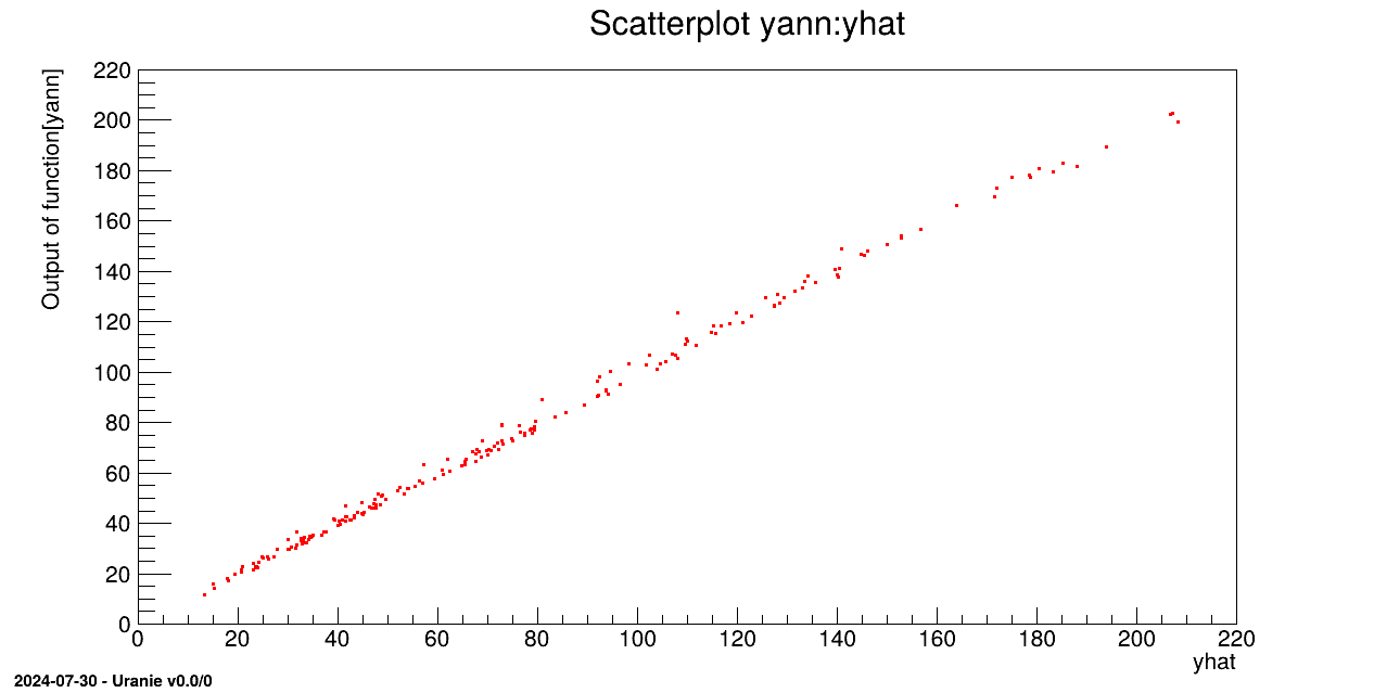
The objective of this macro is to build a surrogate model (an Artificial Neural Network) from a database. From a first database created from an ASCII file flowrate_sampler_launcher_500.dat (which defines values for eight variables described in Section IV.1.2.1 on 500 patterns), two ASCII files are created: one with the 300st patterns (_flowrate_sampler_launcher_app_.dat), the other with the 200 last patterns (_flowrate_sampler_launcher_val_.dat). The surrogate model is built with the database extracted from the first of the two files, the second allowing to perform calculations with a function.

{       
  // Create a TDataServer
  // Load a database in an ASCII file
  TDataServer * tdsu = new TDataServer("tdsu","tds u");
  tdsu->fileDataRead("flowrate_sampler_launcher_500.dat");

  //Create database
  tdsu->exportData("_flowrate_sampler_launcher_app_.dat", "","tdsFlowrate__n__iter__<=300");
  tdsu->exportData("_flowrate_sampler_launcher_val_.dat", "","tdsFlowrate__n__iter__>300");

  TDataServer * tds = new TDataServer("tdsFlowrate", "tds for flowrate");
  tds->fileDataRead("_flowrate_sampler_launcher_app_.dat");
  
  TCanvas *c = new TCanvas("c1", "Graph for the Macro modeler",5,64,1270,667);
  // Buils a surrogate model (Artificial Neural Networks) from the DataBase
  TANNModeler* tann = new TANNModeler(tds, "rw:r:tu:tl:hu:hl:l:kw,3,yhat"); 
  tann->setFcnTol(1e-5);
  //tann->setLog();
  tann->train(3, 2, "test");
  
  tann->exportFunction("pmmlc++","uranie_ann_flowrate","ANNflowrate");
    
  gROOT->LoadMacro("uranie_ann_flowrate.C");

  TDataServer * tdsv = new TDataServer();
  tdsv->fileDataRead("_flowrate_sampler_launcher_val_.dat");

  cout << tdsv->getNPatterns() << endl;

  // evaluate the surrogate model on the database
  TLauncherFunction * tlf = new TLauncherFunction(tdsv, "ANNflowrate", "rw:r:tu:tl:hu:hl:l:kw", "yann");
  tlf->run();    
    
  tdsv->startViewer();
  
  tdsv->Draw("yann:yhat");
  //  tdsv->draw("yhat");
     
}

The main TDataServer loads the main ASCII data file flowrate_sampler_launcher_500.dat

TDataServer * tdsu = new TDataServer("tdsu","tds u");
tdsu->fileDataRead("flowrate_sampler_launcher_500.dat");

The database is split in two parts by exporting the 300st patterns in a file and the remaining 200 in another one:

tdsu->exportData("_flowrate_sampler_launcher_app_.dat", "","tdsFlowrate__n__iter__<=300");
tdsu->exportData("_flowrate_sampler_launcher_val_.dat", "","tdsFlowrate__n__iter__>300");

A second TDataServer loads _flowrate_sampler_launcher_app_.dat and builds the surrogate model over all the variables:

TDataServer * tds = new TDataServer("tds", "tds for flowrate");
tds->fileDataRead("_flowrate_sampler_launcher_app_.dat");
TANNModeler* tann = new TANNModeler(tds, "rw:r:tu:tl:hu:hl:l:kw,3,yhat");
tann->setFcnTol(1e-5);
tann->train(3, 2, "test");

The model is exported in an external file in C++ language "uranie_ann_flowrate.C where the function name is ANNflowrate:

tann->exportFunction("c++", "uranie_ann_flowrate.C","ANNflowrate");

The model is loaded from the macro "uranie_ann_flowrate.C and applied on the second database with the function ANNflowrate:

gROOT->LoadMacro("uranie_ann_flowrate.C");
TDataServer * tdsv = new TDataServer();
tdsv->fileDataRead("_flowrate_sampler_launcher_val_.dat");
TLauncherFunction * tlf = new TLauncherFunction(tdsv, "ANNflowrate", "rw:r:tu:tl:hu:hl:l:kw", "yann");
tlf->run();

Processing modelerFlowrateNeuralNetworks.C...

--- Uranie v0.0/0 --- Developed with ROOT (6.32.02)
                      Copyright (C) 2013-2024 CEA/DES 
                      Contact: support-uranie@cea.fr 
                      Date: Tue Jan 09, 2024

 <URANIE::WARNING> 
 <URANIE::WARNING> *** URANIE WARNING ***
 <URANIE::WARNING> *** File[${SOURCEDIR}/dataSERVER/souRCE/TDataServer.cxx] Line[759]
 <URANIE::WARNING> TDataServer::fileDataRead: Expected iterator tdsu__n__iter__ not found but tdsFlowrate__n__iter__ looks like an URANIE iterator => Will be used as so.
 <URANIE::WARNING> *** END of URANIE WARNING ***
 <URANIE::WARNING> 
 ** TANNModeler::train niter[3] ninit[2]
 ** init the ANN
 ** Input  (1) Name[rw] Min[0.101018] Max[0.0295279]
 ** Input  (2) Name[r] Min[25668.6] Max[14838.3]
 ** Input  (3) Name[tu] Min[89914.4] Max[14909]
 ** Input  (4) Name[tl] Min[89.0477] Max[15.0121]
 ** Input  (5) Name[hu] Min[1048.92] Max[34.8615]
 ** Input  (6) Name[hl] Min[763.058] Max[33.615]
 ** Input  (7) Name[l] Min[1401.09] Max[163.611]
 ** Input  (8) Name[kw] Min[10950.2] Max[635.503]
 ** Output  (1) Name[yhat] Min[78.0931] Max[44.881]
 ** Tolerance  (1e-05)
 ** sHidden    (3) (3)
 ** Nb Weights (31)
 ** ActivationFunction[LOGISTIC]
 **

 ** iter[1/3] : *= : mse_min[0.00150425]
 ** iter[2/3] : ** : mse_min[0.0024702]
 ** iter[3/3] : *= : mse_min[0.00122167]

 ** solutions : 3
 ** isol[1] iter[0] learn[0.00126206] test[0.00150425] *
 ** isol[2] iter[1] learn[0.00152949] test[0.0024702]
 ** isol[3] iter[2] learn[0.00107926] test[0.00122167] *
 ** CPU training finished. Total elapsed time: 1.48 sec

*******************************
*** TModeler::exportFunction lang[pmmlc++] file[uranie_ann_flowrate] name[ANNflowrate] soption[]

*******************************

*******************************
*** exportFunction lang[pmmlc++] file[uranie_ann_flowrate] name[ANNflowrate]

*******************************
PMML Constructor: uranie_ann_flowrate.pmml
*** End Of exportModelPMML 
*******************************
*** End Of exportFunction
*******************************

The objective of this macro is to build a surrogate model (an Artificial Neural Network) from a PMML file.

{
       
  // Create a TDataServer
  // Load a database in an ASCII file
  TDataServer * tds = new TDataServer("tdsFlowrate", "tds for flowrate");
  tds->fileDataRead("_flowrate_sampler_launcher_app_.dat");
    
  TCanvas *c = new TCanvas("c1", "Graph for the Macro modeler",5,64,1270,667);
  // Build a surrogate model (Artificial Neural Networks) from the PMML file
  TANNModeler* tann = new TANNModeler(tds, "uranie_ann_flowrate.pmml","ANNflowrate");
  
  // export the surrogate model in a C file
  tann->exportFunction("c++", "uranie_ann_flowrate_loaded","ANNflowrate");
  // load the surrogate model in the C file
  gROOT->LoadMacro("uranie_ann_flowrate_loaded.C");
 
  TDataServer * tdsv = new TDataServer("tdsv", "tds for surrogate model");
  tdsv->fileDataRead("_flowrate_sampler_launcher_val_.dat");
  
  cout << tdsv->getNPatterns() << endl;

  // evaluate the surrogate model on the database
  TLauncherFunction * tlf = new TLauncherFunction(tdsv, "ANNflowrate", "rw:r:tu:tl:hu:hl:l:kw", "yann");
  tlf->run();
    
  tdsv->startViewer();
  
  tdsv->Draw("yann:yhat");
  //  tdsv->draw("yhat");
   
}

A TDataServer loads _flowrate_sampler_launcher_app_.dat:

TDataServer * tds = new TDataServer("tds", "tds for flowrate");
tds->fileDataRead("_flowrate_sampler_launcher_app_.dat");

The surrogate model is loaded from a PMML file:

TANNModeler* tann = new TANNModeler(tds, "uranie_ann_flowrate.pmml","ANNflowrate");

The model is exported in an external file in C++ language "uranie_ann_flowrate.C where the function name is ANNflowrate:

tann->exportFunction("c++", "uranie_ann_flowrate.C","ANNflowrate");

The model is loaded from the macro "uranie_ann_flowrate.C and applied on the database with the function ANNflowrate:

gROOT->LoadMacro("uranie_ann_flowrate.C");
TDataServer * tdsv = new TDataServer();
tdsv->fileDataRead("_flowrate_sampler_launcher_val_.dat");
TLauncherFunction * tlf = new TLauncherFunction(tdsv, "ANNflowrate", "rw:r:tu:tl:hu:hl:l:kw", "yann");
tlf->run();

Processing modelerFlowrateNeuralNetworksLoadingPMML.C...

--- Uranie v0.0/0 --- Developed with ROOT (6.32.02)
                      Copyright (C) 2013-2024 CEA/DES 
                      Contact: support-uranie@cea.fr 
                      Date: Tue Jan 09, 2024

PMML Constructor: uranie_ann_flowrate.pmml

*******************************
*** TModeler::exportFunction lang[c++] file[uranie_ann_flowrate_loaded] name[ANNflowrate] soption[]

*******************************

*******************************
*** exportFunction lang[c++] file[uranie_ann_flowrate_loaded] name[ANNflowrate]
*** End Of exportFunction
*******************************

The objective of this macro is to build a surrogate model (an Artificial Neural Network) from a database for a "Classification" Problem. From a first database loaded from the ASCII file problem2Classes_001000.dat, which defines three variables 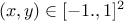and on 1000 patterns,

two ASCII files are created, one with the 800st patterns (_problem2Classes_app_.dat), the other with the 200 last patterns (_problem2Classes_val_.dat). The surrogate model is built with the database extracted from the first of the two files, the second allowing to perform calculations with a function.

{  
    Int_t nH1 = 15;
    Int_t nH2 = 10;
    Int_t nH3 = 5;
    
    TString sX = "x:y";
    TString sY = "rc01";
    TString sYhat = Form("%shat_%d_%d_%d", sY.Data(), nH1, nH2, nH3);

    // Load a database in an ASCII file
    TDataServer * tdsu = new TDataServer("tdsu","tds u");
    tdsu->fileDataRead("problem2Classes_001000.dat");

    // Split into 2 datasets for learning and testing
    tdsu->exportData("_problem2Classes_app_.dat", "", Form("%s<=800", tdsu->getIteratorName()));
    tdsu->exportData("_problem2Classes_val_.dat", "", Form("%s>800", tdsu->getIteratorName()));
    
    TDataServer * tds = new TDataServer("tdsApp", "tds App for problem2Classes");
    tds->fileDataRead("_problem2Classes_app_.dat");

    TANNModeler* tann = new TANNModeler(tds, Form("%s,%d,%d,%d,@%s", sX.Data(), nH1, nH2, nH3, sY.Data())); 
    //tann->setLog();
    tann->setNormalization(TANNModeler::kMinusOneOne);
    tann->setFcnTol(1e-6);
    tann->train(2, 2, "test", kFALSE);
  
    tann->exportFunction("c++","uranie_ann_problem2Classes","ANNproblem2Classes");
    
    gROOT->LoadMacro("uranie_ann_problem2Classes.C");

    TDataServer * tdsv = new TDataServer();
    tdsv->fileDataRead("_problem2Classes_val_.dat");
    
    // evaluate the surrogate model on the database
    TLauncherFunction * tlf = new TLauncherFunction(tdsv, "ANNproblem2Classes", sX, sYhat);
    tlf->run();    
    
    TCanvas *c = new TCanvas("c1", "Graph for the Macro modeler",5,64,1270,667);
    // Buils a surrogate model (Artificial Neural Networks) from the DataBase
    tds->getTuple()->SetMarkerStyle(8);
    tds->getTuple()->SetMarkerSize(1.0);
    tds->getTuple()->SetMarkerColor(kGreen);
    tds->draw(Form("%s:%s", sY.Data(), sX.Data()));
      
    tdsv->getTuple()->SetMarkerStyle(8);
    tdsv->getTuple()->SetMarkerSize(0.75);
    tdsv->getTuple()->SetMarkerColor(kRed);
    tdsv->Draw(Form("%s:%s", sYhat.Data(), sX.Data()),"","same");
     
}

The main TDataServer loads the main ASCII data file problem2Classes_001000.dat

TDataServer * tdsu = new TDataServer("tdsu","tds u");
tdsu->fileDataRead("problem2Classes_001000.dat");

The database is split with the internal iterator attribute in two parts by exporting the 800st patterns in a file and the remaining 200 in another one

tdsu->exportData("_problem2Classes_app_.dat", "",Form("%s<=800", tdsu->getIteratorName()));
tdsu->exportData("_problem2Classes_val_.dat", "", Form("%s>800", tdsu->getIteratorName()));

A second TDataServer loads _problem2Classes_app_.dat and builds the surrogate model over all the variables with 3 hidden layers, a Hyperbolic Tangent (TanH) activation function (normalization) in the 3 hidden layers and set the function tolerance to 1e-.6. The "@" character behind the output name defines a classification problem.

TDataServer * tds = new TDataServer("tds", "tds for the 2 Classes problem");
tds->fileDataRead("_problem2Classes_app_.dat");
TANNModeler* tann = new TANNModeler(tds, Form("%s,%d,%d,%d,@%s", sX.Data(), nH1, nH2, nH3, sY.Data()));
tann->setNormalization(TANNModeler::kMinusOneOne);
tann->setFcnTol(1e-6);
tann->train(3, 2, "test");

The model is exported in an external file in C++ language "uranie_ann_problem2Classes.C" where the function name is ANNproblem2Classes

tann->exportFunction("c++", "uranie_ann_problem2Classes.C","ANNproblem2Classes");

The model is loaded from the macro "uranie_ann_problem2Classes.C and applied on the second database with the function ANNproblem2Classes.

gROOT->LoadMacro("uranie_ann_problem2Classes.C");
TDataServer * tdsv = new TDataServer();
tdsv->fileDataRead("_problem2Classes_val_.dat");
TLauncherFunction * tlf = new TLauncherFunction(tdsv, "ANNproblem2Classes", sX, sYhat);
tlf->run();

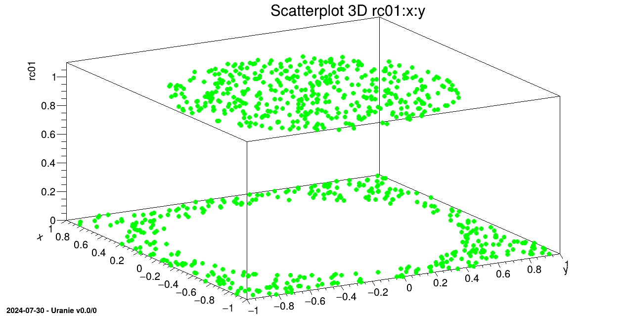
We draw on a 3D graph, the learning database (in green) and the estimations by the Artificial Neural Network with red points.

TCanvas *c = new TCanvas("c1", "Graph for the Macro modeler",5,64,1270,667);
tds->getTuple()->SetMarkerStyle(8);
tds->getTuple()->SetMarkerSize(1.0);
tds->getTuple()->SetMarkerColor(kGreen);
tds->draw(Form("%s:%s", sY.Data(), sX.Data()));

tdsv->getTuple()->SetMarkerStyle(8);
tdsv->getTuple()->SetMarkerSize(0.75);
tdsv->getTuple()->SetMarkerColor(kRed);
tdsv->Draw(Form("%s:%s", sYhat.Data(), sX.Data()),"","same");
	

Processing modelerClassificationNeuralNetworks.C...

--- Uranie v0.0/0 --- Developed with ROOT (6.32.02)
                      Copyright (C) 2013-2024 CEA/DES 
                      Contact: support-uranie@cea.fr 
                      Date: Tue Jan 09, 2024

 <URANIE::WARNING> 
 <URANIE::WARNING> *** URANIE WARNING ***
 <URANIE::WARNING> *** File[${SOURCEDIR}/dataSERVER/souRCE/TDataServer.cxx] Line[759]
 <URANIE::WARNING> TDataServer::fileDataRead: Expected iterator tdsu__n__iter__ not found but _tds___n__iter__ looks like an URANIE iterator => Will be used as so.
 <URANIE::WARNING> *** END of URANIE WARNING ***
 <URANIE::WARNING> 
 <URANIE::WARNING> 
 <URANIE::WARNING> *** URANIE WARNING ***
 <URANIE::WARNING> *** File[${SOURCEDIR}/dataSERVER/souRCE/TDataServer.cxx] Line[759]
 <URANIE::WARNING> TDataServer::fileDataRead: Expected iterator tdsApp__n__iter__ not found but _tds___n__iter__ looks like an URANIE iterator => Will be used as so.
 <URANIE::WARNING> *** END of URANIE WARNING ***
 <URANIE::WARNING> 
 ** TANNModeler::train niter[2] ninit[2]
 ** init the ANN
 ** Input  (1) Name[x] Min[-0.999842] Max[0.998315]
 ** Input  (2) Name[y] Min[-0.999434] Max[0.998071]
 ** Output  (1) Name[rc01] Min[0] Max[1]
 ** Tolerance  (1e-06)
 ** sHidden    (15,10,5) (30)
 ** Nb Weights (266)
 ** ActivationFunction[TanH]
 **

 ** iter[1/2] : ** : mse_min[0.00813999]
 ** iter[2/2] : ** : mse_min[0.00636923]

 ** solutions : 2
 ** isol[1] iter[0] learn[0.00405863] test[0.00813999] *
 ** isol[2] iter[1] learn[0.00560685] test[0.00636923] *
 ** CPU training finished. Total elapsed time: 16.7 sec

*******************************
*** TModeler::exportFunction lang[c++] file[uranie_ann_problem2Classes] name[ANNproblem2Classes] soption[]

*******************************

*******************************
*** exportFunction lang[c++] file[uranie_ann_problem2Classes] name[ANNproblem2Classes]
*** End Of exportFunction
*******************************

The objective of this macro is to build a polynomial chaos expansion in order to get a surrogate model along with a global sensitivity interpretation for the flowrate function, whose purpose and behaviour have been already introduced in Section IV.1.2.1. The method used here is the regression one, as discussed below.

{

    gROOT->LoadMacro("UserFunctions.C");
  
    // Define the DataServer
    TDataServer *tds = new TDataServer("tdsFlowrate", "Design of experiments for Flowrate");
    // Add the eight attributes of the study with uniform law
    tds->addAttribute( new TUniformDistribution("rw", 0.05, 0.15));
    tds->addAttribute( new TUniformDistribution("r", 100.0, 50000.0));
    tds->addAttribute( new TUniformDistribution("tu", 63070.0, 115600.0));
    tds->addAttribute( new TUniformDistribution("tl", 63.1, 116.0));
    tds->addAttribute( new TUniformDistribution("hu", 990.0, 1110.0));
    tds->addAttribute( new TUniformDistribution("hl", 700.0, 820.0));
    tds->addAttribute( new TUniformDistribution("l", 1120.0, 1680.0));
    tds->addAttribute( new TUniformDistribution("kw", 9855.0, 12045.0));         
  
    // Define of TNisp object
    TNisp *nisp = new TNisp(tds);
    nisp->generateSample("QmcSobol", 500); //State that there is a sample ...

    // Compute the output variable
    TLauncherFunction * tlf = new TLauncherFunction(tds, "flowrateModel","*","ymod");
    tlf->setDrawProgressBar(kFALSE);
    tlf->run();
    
    // build a chaos polynomial
    TPolynomialChaos *pc = new TPolynomialChaos(tds,nisp); 

    // compute the pc coefficients using the "Regression" method
    Int_t degree = 4;
    pc->setDegree(degree);
    pc->computeChaosExpansion("Regression");
  
    // Uncertainty and sensitivity analysis
    cout << "Variable ymod ================" << endl;
    cout << "Mean     = " << pc->getMean("ymod") << endl;
    cout << "Variance = " << pc->getVariance("ymod") << endl;
    cout << "First Order Indices ================" << endl;
    cout << "Indice First Order[1] = " <<  pc->getIndexFirstOrder(0,0) << endl;
    cout << "Indice First Order[2] = " <<  pc->getIndexFirstOrder(1,0) << endl;
    cout << "Indice First Order[3] = " <<  pc->getIndexFirstOrder(2,0) << endl;
    cout << "Indice First Order[4] = " <<  pc->getIndexFirstOrder(3,0) << endl;
    cout << "Indice First Order[5] = " <<  pc->getIndexFirstOrder(4,0) << endl;
    cout << "Indice First Order[6] = " <<  pc->getIndexFirstOrder(5,0) << endl;
    cout << "Indice First Order[7] = " <<  pc->getIndexFirstOrder(6,0) << endl;
    cout << "Indice First Order[8] = " <<  pc->getIndexFirstOrder(7,0) << endl;
    cout << "Total Order Indices ================" << endl;
    cout << "Indice Total Order[1] = " << pc->getIndexTotalOrder("rw","ymod") << endl;
    cout << "Indice Total Order[2] = " << pc->getIndexTotalOrder("r","ymod") << endl;
    cout << "Indice Total Order[3] = " << pc->getIndexTotalOrder("tu","ymod") << endl;
    cout << "Indice Total Order[4] = " << pc->getIndexTotalOrder("tl","ymod") << endl;
    cout << "Indice Total Order[5] = " << pc->getIndexTotalOrder("hu","ymod") << endl;
    cout << "Indice Total Order[6] = " << pc->getIndexTotalOrder("hl","ymod") << endl;
    cout << "Indice Total Order[7] = " << pc->getIndexTotalOrder("l","ymod") << endl;
    cout << "Indice Total Order[8] = " << pc->getIndexTotalOrder("kw","ymod") << endl;

    // Dump main factors up to a certain threshold
    Double_t seuil = 0.99;
    cout<<"Ordered functionnal ANOVA"<<endl;
    pc->getAnovaOrdered(seuil,0);

    cout << "Number of experiments = " << tds->getNPatterns() << endl;

    //save the pv in a program (C langage)
    pc->exportFunction("NispFlowrate","NispFlowrate");
      
}

The first part is just creating a TDataServer and providing the attributes needed to define the problem. From there, a TNisp object is created, providing the dataserver that specifies the inputs. This class is used to generate the sample.

// Define of TNisp object
TNisp *nisp = new TNisp(tds);
nisp->generateSample("QmcSobol", 500); //State that there is a sample ... 

The function is launched through a TLauncherFunction instance in order to get the output values that will be needed to train the surrogate model.

TLauncherFunction * tlf = new TLauncherFunction(tds, "flowrateModel","*","ymod");
tlf->run();

Finally, a TPolynomialChaos instance is created and the computation of the coefficients is performed by requesting a truncature on the resulting degree of the polynomial expansion (set to 4) and the use of a regression method.

// build a chaos polynomial
TPolynomialChaos *pc = new TPolynomialChaos(tds,nisp); 
// compute the pc coefficients using the "Regression" method
Int_t degree = 4;
pc->setDegree(degree);
pc->computeChaosExpansion("Regression");

The rest of the code is showing how to access the resulting sensitivity indices either one-by-one, or ordered up to a chosen threshold of the output variance.

Processing modelerFlowratePolynChaosRegression.C...

--- Uranie v0.0/0 --- Developed with ROOT (6.32.02)
                      Copyright (C) 2013-2024 CEA/DES 
                      Contact: support-uranie@cea.fr 
                      Date: Tue Jan 09, 2024

Variable ymod ================
Mean     = 77.651
Variance = 2079.68
First Order Indices ================
Indice First Order[1] = 0.828732
Indice First Order[2] = 1.05548e-06
Indice First Order[3] = 9.86805e-08
Indice First Order[4] = 4.77668e-06
Indice First Order[5] = 0.0414015
Indice First Order[6] = 0.0413215
Indice First Order[7] = 0.039401
Indice First Order[8] = 0.00954644
Total Order Indices ================
Indice Total Order[1] = 0.866773
Indice Total Order[2] = 9.27467e-06
Indice Total Order[3] = 7.01768e-06
Indice Total Order[4] = 1.71944e-05
Indice Total Order[5] = 0.0541916
Indice Total Order[6] = 0.0540578
Indice Total Order[7] = 0.0522121
Indice Total Order[8] = 0.0127809

The objective of this macro is to build a polynomial chaos expansion in order to get a surrogate model along with a global sensitivity interpretation for the flowrate function, whose purpose and behaviour have been already introduced in Section IV.1.2.1. The method used here is the regression one, as discussed below.

{

    gROOT->LoadMacro("UserFunctions.C");
  
    // Define the DataServer
    TDataServer *tds = new TDataServer("tdsFlowrate", "Design of experiments for Flowrate");
    // Add the eight attributes of the study with uniform law
    tds->addAttribute( new TUniformDistribution("rw", 0.05, 0.15));
    tds->addAttribute( new TUniformDistribution("r", 100.0, 50000.0));
    tds->addAttribute( new TUniformDistribution("tu", 63070.0, 115600.0));
    tds->addAttribute( new TUniformDistribution("tl", 63.1, 116.0));
    tds->addAttribute( new TUniformDistribution("hu", 990.0, 1110.0));
    tds->addAttribute( new TUniformDistribution("hl", 700.0, 820.0));
    tds->addAttribute( new TUniformDistribution("l", 1120.0, 1680.0));
    tds->addAttribute( new TUniformDistribution("kw", 9855.0, 12045.0));         
  
    // Define of TNisp object
    TNisp *nisp = new TNisp(tds);
    nisp->generateSample("Petras", 5); //State that there is a sample ...

    // Compute the output variable
    TLauncherFunction * tlf = new TLauncherFunction(tds, "flowrateModel","*","ymod");
    tlf->setDrawProgressBar(kFALSE);
    tlf->run();
    
    // build a chaos polynomial
    TPolynomialChaos *pc = new TPolynomialChaos(tds,nisp); 

    // compute the pc coefficients using the "Integration" method
    Int_t degree = 4;
    pc->setDegree(degree);
    pc->computeChaosExpansion("Integration");
  
    // Uncertainty and sensitivity analysis
    cout << "Variable ymod ================" << endl;
    cout << "Mean     = " << pc->getMean("ymod") << endl;
    cout << "Variance = " << pc->getVariance("ymod") << endl;
    cout << "First Order Indices ================" << endl;
    cout << "Indice First Order[1] = " <<  pc->getIndexFirstOrder(0,0) << endl;
    cout << "Indice First Order[2] = " <<  pc->getIndexFirstOrder(1,0) << endl;
    cout << "Indice First Order[3] = " <<  pc->getIndexFirstOrder(2,0) << endl;
    cout << "Indice First Order[4] = " <<  pc->getIndexFirstOrder(3,0) << endl;
    cout << "Indice First Order[5] = " <<  pc->getIndexFirstOrder(4,0) << endl;
    cout << "Indice First Order[6] = " <<  pc->getIndexFirstOrder(5,0) << endl;
    cout << "Indice First Order[7] = " <<  pc->getIndexFirstOrder(6,0) << endl;
    cout << "Indice First Order[8] = " <<  pc->getIndexFirstOrder(7,0) << endl;
    cout << "Total Order Indices ================" << endl;
    cout << "Indice Total Order[1] = " << pc->getIndexTotalOrder("rw","ymod") << endl;
    cout << "Indice Total Order[2] = " << pc->getIndexTotalOrder("r","ymod") << endl;
    cout << "Indice Total Order[3] = " << pc->getIndexTotalOrder("tu","ymod") << endl;
    cout << "Indice Total Order[4] = " << pc->getIndexTotalOrder("tl","ymod") << endl;
    cout << "Indice Total Order[5] = " << pc->getIndexTotalOrder("hu","ymod") << endl;
    cout << "Indice Total Order[6] = " << pc->getIndexTotalOrder("hl","ymod") << endl;
    cout << "Indice Total Order[7] = " << pc->getIndexTotalOrder("l","ymod") << endl;
    cout << "Indice Total Order[8] = " << pc->getIndexTotalOrder("kw","ymod") << endl;

    // Dump main factors up to a certain threshold
    Double_t seuil = 0.99;
    cout<<"Ordered functionnal ANOVA"<<endl;
    pc->getAnovaOrdered(seuil,0);

    cout << "Number of experiments = " << tds->getNPatterns() << endl;

    //save the pv in a program (C langage)
    pc->exportFunction("NispFlowrate","NispFlowrate");
      
}

The first part is just creating a TDataServer and providing the attributes needed to define the problem. From there, a TNisp object is created, providing the dataserver that specifies the inputs. This class is used to generate the sample (Petras being a design-of-experiments dedicated to integration problem).

// Define of TNisp object
TNisp *nisp = new TNisp(tds);
nisp->generateSample("Petras", 5); //State that there is a sample ... 

The function is launched through a TLauncherFunction instance in order to get the output values that will be needed to train the surrogate model.

TLauncherFunction * tlf = new TLauncherFunction(tds, "flowrateModel","*","ymod");
tlf->run();

Finally, a TPolynomialChaos instance is created and the computation of the coefficients is performed by requesting a truncature on the resulting degree of the polynomial expansion (set to 4) and the use of a regression method.

// build a chaos polynomial
TPolynomialChaos *pc = new TPolynomialChaos(tds,nisp); 
// compute the pc coefficients using the "Integration" method
Int_t degree = 4;
pc->setDegree(degree);
pc->computeChaosExpansion("Integration");

The rest of the code is showing how to access the resulting sensitivity indices either one-by-one, or ordered up to a chosen threshold of the output variance.

Processing modelerFlowratePolynChaosIntegration.C...

--- Uranie v0.0/0 --- Developed with ROOT (6.32.02)
                      Copyright (C) 2013-2024 CEA/DES 
                      Contact: support-uranie@cea.fr 
                      Date: Tue Jan 09, 2024

Variable ymod ================
Mean     = 77.6511
Variance = 2078.91
First Order Indices ================
Indice First Order[1] = 0.828922
Indice First Order[2] = 1.04477e-06
Indice First Order[3] = 8.94692e-12
Indice First Order[4] = 5.30299e-06
Indice First Order[5] = 0.0413852
Indice First Order[6] = 0.0413852
Indice First Order[7] = 0.0393419
Indice First Order[8] = 0.00952157
Total Order Indices ================
Indice Total Order[1] = 0.866834
Indice Total Order[2] = 2.16178e-06
Indice Total Order[3] = 2.28296e-09
Indice Total Order[4] = 1.07386e-05
Indice Total Order[5] = 0.0541095
Indice Total Order[6] = 0.0541095
Indice Total Order[7] = 0.0520767
Indice Total Order[8] = 0.0127306

This macro is the one described in Section V.6.2.2, that creates a simple gaussian process, whose training (utf_4D_train.dat) and testing (utf_4D_test.dat) database can both be found in the document folder of the Uranie installation (${URANIESYS}/share/uranie/docUMENTS).

{
  // Load observations
  TDataServer *tdsObs = new TDataServer("tdsObs", "observations");
  tdsObs->fileDataRead("utf_4D_train.dat");
	
  // Construct the GPBuilder
  TGPBuilder *gpb = new TGPBuilder(tdsObs,            // observations data 
				   "x1:x2:x3:x4",     // list of input variables
				   "y",               // output variable
				   "matern3/2");      // name of the correlation function

  
  // Search for the optimal hyper-parameters
  gpb->findOptimalParameters("ML",            // optimisation criterion 
			     100,             // screening design size
			     "neldermead",    // optimisation algorithm
			     500);            // max. number of optimisation iterations
	
  // Construct the kriging model
  TKriging *krig = gpb->buildGP();
	
  // Display model information
  krig->printLog();

  }

This is the result of the last command:

*******************************
** TKriging::printLog[]
*******************************
 Input Variables:      x1:x2:x3:x4
 Output Variable:      y
 Deterministic trend:  
 Correlation function: URANIE::Modeler::TMatern32CorrFunction
 Correlation length:   normalised   (not normalised)
                       1.6181e+00 (1.6172e+00 )
                       1.4372e+00 (1.4370e+00 )
                       1.5026e+00 (1.5009e+00 )
                       6.7884e+00 (6.7944e+00 )

 Variance of the gaussian process:      70.8755
 RMSE (by Leave One Out):               0.499108
 Q2:                                    0.849843
*******************************

This macro is the one described in Section V.6.2.7, that creates a gaussian process, whose training (utf_4D_train.dat) and testing (utf_4D_test.dat) database can both be found in the document folder of the Uranie installation (${URANIESYS}/share/uranie/docUMENTS), and whose starting point, in the parameter space, is specified.

{
 // Load observations
 TDataServer *tdsObs = new TDataServer("tdsObs", "observations");
 tdsObs->fileDataRead("utf_4D_train.dat");
 
 // Construct the GPBuilder
 TGPBuilder *gpb = new TGPBuilder(tdsObs, "x1:x2:x3:x4", "y", "matern3/2");
 
 // Set the correlation function parameters
 Double_t params[4] = {1.0, 0.25, 0.01, 0.3};
 gpb->getCorrFunction()->setParameters(params);

 // Find the optimal parameters
 gpb->findOptimalParameters("ML",         // optimisation criterion 
                            0,            // screening size MUST be equal to 0 
			    "neldermead", // optimisation algorithm
			    500,          // max. number of optimisation iterations
			    kFALSE);      // we don't reset the parameters of the GP builder
      
  // Create the kriging model
  TKriging *krig = gpb->buildGP();
      
  // Display model information
  krig->printLog();                

  }

This is the result of the last command:

*******************************
** TKriging::printLog[]
*******************************
 Input Variables:      x1:x2:x3:x4
 Output Variable:      y
 Deterministic trend:  
 Correlation function: URANIE::Modeler::TMatern32CorrFunction
 Correlation length:   normalised   (not normalised)
                       1.6182e+00 (1.6173e+00 )
                       1.4373e+00 (1.4371e+00 )
                       1.5027e+00 (1.5011e+00 )
                       6.7895e+00 (6.7955e+00 )

 Variance of the gaussian process:      70.8914
 RMSE (by Leave One Out):               0.49911
 Q2:                                    0.849842
*******************************

This macro is the one described in Section V.6.2.4, that creates a gaussian process with a specific trend and an a priori knowledge on the mean and variance of the trend parameters.

{
    // Load observations
   TDataServer *tdsObs = new TDataServer("tdsObs", "observations");
   tdsObs->fileDataRead("utf_4D_train.dat");
  
   // Construct the GPBuilder
   TGPBuilder *gpb = new TGPBuilder(tdsObs,            // observations data 
				    "x1:x2:x3:x4",     // list of input variables
				    "y",               // output variable
				    "matern3/2",       // name of the correlation function
				    "linear");         // trend defined by a keyword


   // Bayesian study
   Double_t meanPrior[5] = {0.0, 0.0, -1.0, 0.0, -0.1};
   Double_t covPrior[25] = {1e-4, 0.0 , 0.0 , 0.0 , 0.0 ,
			    0.0 , 1e-4, 0.0 , 0.0 , 0.0 ,
			    0.0 , 0.0 , 1e-4, 0.0 , 0.0 ,
			    0.0 , 0.0 , 0.0 , 1e-4, 0.0 ,
			    0.0 , 0.0 , 0.0 , 0.0 , 1e-4};
   gpb->setPriorData(meanPrior, covPrior);                                 
	
   // Search for the optimal hyper-parameters
   gpb->findOptimalParameters("ReML",          // optimisation criterion 
			      100,             // screening design size
			      "neldermead",    // optimisation algorithm
			      500);            // max. number of optimisation iterations
	
   // Construct the kriging model
   TKriging *krig = gpb->buildGP();
	
   // Display model information
   krig->printLog();

  }

This is the result of the last command:

*******************************
** TKriging::printLog[]
*******************************
 Input Variables:      x1:x2:x3:x4
 Output Variable:      y
 Deterministic trend:  linear
 Trend parameters (5): [3.06586494e-05; 1.64887174e-05; -9.99986787e-01; 1.51959859e-05; -9.99877606e-02 ]
 Correlation function: URANIE::Modeler::TMatern32CorrFunction
 Correlation length:   normalised   (not normalised)
                       2.1450e+00 (2.1438e+00 )
                       1.9092e+00 (1.9090e+00 )
                       2.0062e+00 (2.0040e+00 )
                       8.4315e+00 (8.4390e+00 )

 Variance of the gaussian process:      155.533
 RMSE (by Leave One Out):               0.495448
 Q2:                                    0.852037
*******************************

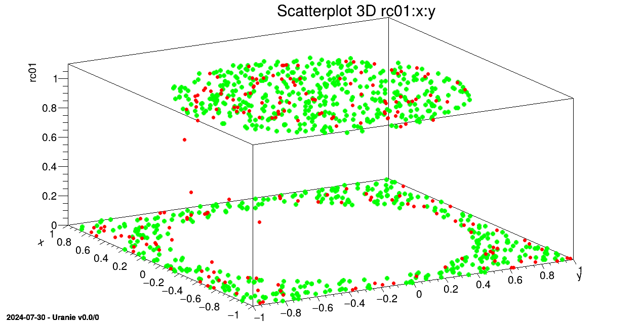
This macro is the one described in Section V.6.3.1, to create and use a simple gaussian process, whose training (utf_4D_train.dat) and testing (utf_4D_test.dat) database can both be found in the document folder of the Uranie installation (${URANIESYS}/share/uranie/docUMENTS). It uses the simple one-by-one approch described in the [metho] for completness.

{
  // Load observations
  TDataServer *tdsObs = new TDataServer("tdsObs", "observations");
  tdsObs->fileDataRead("utf_4D_train.dat");
      
  // Construct the GPBuilder
  TGPBuilder *gpb = new TGPBuilder(tdsObs,            // observations data 
				   "x1:x2:x3:x4",     // list of input variables
				   "y",               // output variable
				   "matern3/2");       // name of the correlation function

                    
  // Search for the optimal hyper-parameters
  gpb->findOptimalParameters("ML",            // optimisation criterion 
			     100,             // screening design size
			     "neldermead",    // optimisation algorithm
			     500);            // max. number of optimisation iterations
      
  // Construct the kriging model
  TKriging *krig = gpb->buildGP();
      
  // Display model information
  krig->printLog();
      
  // Load the data to estimate
  TDataServer *tdsEstim = new TDataServer("tdsEstim", "estimations");
  tdsEstim->fileDataRead("utf_4D_test.dat");
      
  // Construction of the launcher
  TLauncher2 *lanceur = new TLauncher2(tdsEstim,          // data to estimate
				       krig,              // model used for the estimation
				       "x1:x2:x3:x4",     // list of the input variables
				       "yEstim:vEstim");  // name given to the model's outputs 
      
  // Launch the estimations
  lanceur->solverLoop();
      
  // Display some results
  tdsEstim->draw("yEstim:y");

  }

This macro is the one described in Section V.6.3.2, to create and use a simple gaussian process, whose training (utf_4D_train.dat) and testing (utf_4D_test.dat) database can both be found in the document folder of the Uranie installation (${URANIESYS}/share/uranie/docUMENTS). It uses the global approach, computing the input covariance matrix and translating it to the prediction covariance matrix.

{
  // Load observations
  TDataServer *tdsObs = new TDataServer("tdsObs", "observations");
  tdsObs->fileDataRead("utf_4D_train.dat");
      
  // Construct the GPBuilder
  TGPBuilder *gpb = new TGPBuilder(tdsObs,            // observations data 
				   "x1:x2:x3:x4",     // list of input variables
				   "y",               // output variable
				   "matern1/2");       // name of the correlation function

                    
  // Search for the optimal hyper-parameters
  gpb->findOptimalParameters("ML",            // optimisation criterion 
			     100,             // screening design size
			     "neldermead",    // optimisation algorithm
			     500);            // max. number of optimisation iterations
      
  // Construct the kriging model
  TKriging *krig = gpb->buildGP();
      
  // Display model information
  krig->printLog();
      
  // Load the data to estimate
  TDataServer *tdsEstim = new TDataServer("tdsEstim", "estimations");
  tdsEstim->fileDataRead("utf_4D_test.dat");

  // Reducing the database to 1000 first event (prediction cov matrix of a million value !)
  int nST=1000;
  tdsEstim->exportData("utf_4D_test_red.dat","",Form("tdsEstim__n__iter__<=%d",nST));
  tdsEstim->fileDataRead("utf_4D_test_red.dat",false,true); // Reload reduce sample    

 krig->estimateWithCov(tdsEstim, // data to estimate
                        "x1:x2:x3:x4",// list of the input variables
                        "yEstim:vEstim", // name given to the model's outputs
                        "y", //name of the true reference if validation database
                        ""); //options

  TCanvas *c2=NULL;
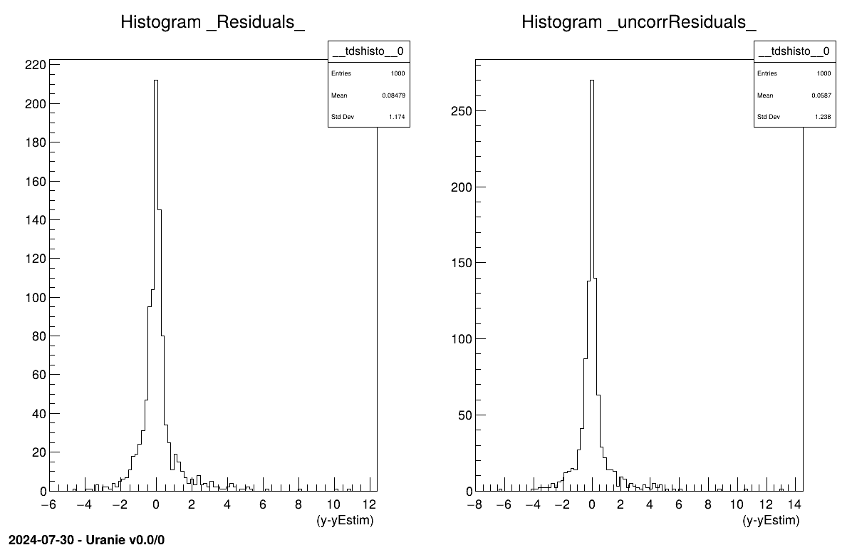
  // Residuals plots if true information provided
  if( tdsEstim->isAttribute("_Residuals_") ) 
  {
      c2 = new TCanvas("c2","c2",1200,800);
      c2->Divide(2,1);
      c2->cd(1);
      // Usual residual considering uncorrated input points
      tdsEstim->Draw("_Residuals_"); 
      c2->cd(2);
      // Corrected residuals, with prediction covariance matrix
      tdsEstim->Draw("_uncorrResiduals_"); 
  }

  // Retrieve all the prediction covariance coefficient
  tdsEstim->getTuple()->SetEstimate( nST * nST ); //allocate the correct size
  // Get a pointer to all values
  tdsEstim->getTuple()->Draw("_CovarianceMatrix_","","goff");
  double *cov=tdsEstim->getTuple()->GetV1();

  //Put these in a matrix nicely created
  TMatrixD Cov(nST,nST);
  Cov.Use(0,nST-1,0,nST-1,cov);

  //Print it if size is reasonnable
  if(nST<10)
      Cov.Print();

  }

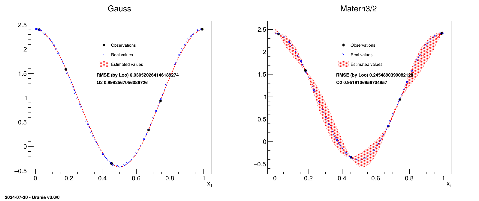
The idea is to provide a simple example of a kriging usage, and an how to, to produce plots in one dimension to represent the results. This example is the one taken from [metho] that uses a very simple set of six points as training database:

#TITLE: utf-1D-train.dat
#COLUMN_NAMES: x1|y

6.731290e-01 3.431918e-01
7.427596e-01 9.356860e-01
4.518467e-01 -3.499771e-01
2.215734e-02 2.400531e+00
9.915253e-01 2.412209e+00
1.815769e-01 1.589435e+00

The aim will be to get a kriging model that describes this dataset and to check its consistency over a certain number of points (here 100 points) which will be the testing database:

#TITLE: utf-1D-test.dat
#COLUMN_NAMES: x1|y

5.469435e-02 2.331524e+00
3.803054e-01 -3.277316e-02
7.047152e-01 6.030177e-01
2.360045e-02 2.398694e+00
9.271965e-01 2.268814e+00
7.868263e-01 1.324318e+00
7.791920e-01 1.257942e+00
6.107965e-01 -8.514510e-02
1.362316e-01 1.926999e+00
5.709913e-01 -2.758435e-01
8.738804e-01 1.992941e+00
2.251602e-01 1.219826e+00
9.175259e-01 2.228545e+00
5.128368e-01 -4.096161e-01
7.692913e-01 1.170999e+00
7.394406e-01 9.062407e-01
5.364506e-01 -3.772856e-01
1.861864e-01 1.551961e+00
7.573444e-01 1.065237e+00
1.005755e-01 2.141109e+00
9.114685e-01 2.201001e+00
3.628465e-01 7.920271e-02
2.383583e-01 1.103353e+00
7.468092e-01 9.716492e-01
3.126209e-01 4.578112e-01
8.034716e-01 1.466248e+00
6.730402e-01 3.424931e-01
8.021345e-01 1.455015e+00
2.503736e-01 9.966807e-01
9.001793e-01 2.145059e+00
7.019990e-01 5.799112e-01
6.001746e-01 -1.432102e-01
4.925013e-01 -4.126441e-01
5.685795e-01 -2.849419e-01
1.238257e-01 2.007351e+00
2.825838e-01 7.124861e-01
4.025708e-01 -1.574002e-01
8.562999e-01 1.875879e+00
3.214125e-01 3.865241e-01
2.021767e-01 1.418581e+00
6.338581e-01 5.717657e-02
3.042007e-01 5.276410e-01
4.860707e-01 -4.088007e-01
9.645326e-01 2.379243e+00
3.583711e-02 2.378513e+00
2.143110e-01 1.314473e+00
7.299624e-01 8.224203e-01
2.719263e-02 2.393622e+00
3.321495e-01 3.020224e-01
8.642671e-01 1.930341e+00
8.893604e-01 2.086039e+00
1.119469e-01 2.078562e+00
9.859741e-01 2.408725e+00
5.594688e-01 -3.166326e-01
1.904448e-01 1.516930e+00
4.232618e-01 -2.529865e-01
1.402221e-01 1.899932e+00
2.647519e-01 8.691058e-01
1.667035e-01 1.706823e+00
2.332246e-01 1.148786e+00
8.324190e-01 1.700059e+00
4.743443e-01 -3.958790e-01
3.435927e-01 2.154677e-01
9.846049e-01 2.407603e+00
9.705327e-01 2.390043e+00
6.631883e-01 2.662970e-01
6.153726e-01 -5.862472e-02
4.632361e-01 -3.766509e-01
6.474053e-01 1.502050e-01
7.161034e-02 2.273461e+00
4.514511e-01 -3.489255e-01
5.976782e-02 2.315661e+00
8.361934e-01 1.729000e+00
5.280981e-01 -3.922313e-01
9.394759e-01 2.313181e+00
2.710088e-01 8.138628e-01
8.161943e-01 1.571375e+00
5.047683e-01 -4.135789e-01
8.427635e-02 2.220534e+00
3.540224e-01 1.400987e-01
4.698548e-03 2.413597e+00
9.124315e-02 2.188105e+00
9.996285e-01 2.414210e+00
4.167139e-01 -2.249546e-01
5.892062e-01 -1.978247e-01
2.929336e-01 6.231119e-01
4.456454e-01 -3.325379e-01
1.148699e-02 2.410532e+00
3.892636e-01 -8.548741e-02
7.188374e-01 7.248622e-01
3.697949e-01 3.323350e-02
6.864519e-01 4.502113e-01
1.586679e-01 1.767741e+00
6.603030e-01 2.445009e-01
6.277168e-01 1.721489e-02
4.305704e-01 -2.817686e-01
1.553435e-01 1.792379e+00
5.476842e-01 -3.512131e-01
8.475444e-01 1.813503e+00
9.527370e-01 2.352313e+00

In this example, two different correlation functions are tested and the obtained results are compared at the end.

void PrintSolutions(TDataServer *tdsObs, TDataServer *tdsEstim, string title) 
{

  const int nbObs = tdsObs->getNPatterns();
  const int nbEst = tdsEstim->getNPatterns();
  vector<double> Rxarr(nbEst,0), x_arr(nbEst,0), y_est(nbEst,0), y_rea(nbEst,0), std_var(nbEst,0);
  
  tdsEstim->computeRank("x1");
  tdsEstim->getTuple()->copyBranchData(&Rxarr[0],nbEst,"Rk_x1");
  tdsEstim->getTuple()->copyBranchData(&x_arr[0],nbEst,"x1");
  tdsEstim->getTuple()->copyBranchData(&y_est[0],nbEst,"yEstim");
  tdsEstim->getTuple()->copyBranchData(&y_rea[0],nbEst,"y");
  tdsEstim->getTuple()->copyBranchData(&std_var[0],nbEst,"vEstim");
  
  vector<double> xarr(nbEst,0), yest(nbEst,0), yrea(nbEst,0), stdvar(nbEst,0);
  int ind;
  for (int i=0; i<nbEst; i++)
  {
    ind = int(Rxarr[i]) - 1;
    xarr[ind] = x_arr[i];
    yest[ind] = y_est[i];
    yrea[ind] = y_rea[i];
    stdvar[ind] = 2*sqrt(fabs(std_var[i]));
  }

  vector<double> xobs(nbObs,0); tdsObs->getTuple()->copyBranchData(&xobs[0],nbObs,"x1");
  vector<double> yobs(nbObs,0); tdsObs->getTuple()->copyBranchData(&yobs[0],nbObs,"y");

  TGraph *gobs = new TGraph(nbObs,&xobs[0],&yobs[0]);
  gobs->SetMarkerColor(1); gobs->SetMarkerSize(1); gobs->SetMarkerStyle(8);
  TGraphErrors *gest = new TGraphErrors(nbEst,&xarr[0],&yest[0],0,&stdvar[0]);
  gest->SetLineColor(2); gest->SetLineWidth(1); gest->SetFillColor(2); gest->SetFillStyle(3002); 
  TGraph *grea = new TGraph(nbEst,&xarr[0],&yrea[0]);
  grea->SetMarkerColor(4); grea->SetMarkerSize(1); grea->SetMarkerStyle(5); grea->SetTitle("Real Values");

  TMultiGraph *mg = new TMultiGraph("toto", title.c_str());
  mg->Add(gest,"l3"); mg->Add(gobs,"P"); mg->Add(grea,"P");
  mg->Draw("A");
  mg->GetXaxis()->SetTitle("x_{1}");

  TLegend *leg= new TLegend(0.4,0.65,0.65,0.8);
  leg->AddEntry(gobs, "Observations", "p");
  leg->AddEntry(grea, "Real values", "p");
  leg->AddEntry(gest, "Estimated values", "lf");
  leg->Draw();
}


void modelerTestKriging()
{
  //Create dataserver and read training database
  TDataServer *tdsObs = new TDataServer("tdsObs","observations"); 
  tdsObs->fileDataRead("utf-1D-train.dat");
  const int nbObs = 6; 

  // Canvas, divided in 2
  TCanvas *Can = new TCanvas("can","can",10,32,1600,700);
  TPad *apad = new TPad("apad","apad",0, 0.03, 1, 1);
  apad->Draw(); apad->Divide(2,1);
  
  //Name of the plot and correlation functions used
  string outplot="GaussAndMatern_1D_AllPoints.png";
  string Correl[2] = {"Gauss","Matern3/2"};

  //Pointer to needed objects, created in the loop
  TGPBuilder *gpb[2];
  TKriging *kg[2];
  TDataServer *tdsEstim[2];
  TLauncher2 *lkrig[2];

  stringstream sstr;
  //Looping over the two correlation function chosen
  for (int imet=0; imet<2; imet++)
  { 
    //Create the TGPBuiler object with chosen option and find optimal parameters
    gpb[imet] = new TGPBuilder(tdsObs, "x1", "y", Correl[imet].c_str(), "");
    gpb[imet]->findOptimalParameters("LOO", 100, "Subplexe", 1000);

    //Get the kriging object
    kg[imet] = gpb[imet]->buildGP();

    //open the dataserver and read the testing basis
    sstr.str(""); sstr << "tdsEstim_" << imet;
    tdsEstim[imet] = new TDataServer(sstr.str().c_str(),"base de test");
    tdsEstim[imet]->fileDataRead("utf-1D-test.dat");
    
    //applied resulting kriging on test basis
    lkrig[imet] = new TLauncher2(tdsEstim[imet], kg[imet], "x1", "yEstim:vEstim");
    lkrig[imet]->solverLoop();
    
    //do the plot
    apad->cd(imet+1);
    PrintSolutions(tdsObs, tdsEstim[imet], Correl[imet]);
    
    stringstream sstr; TLatex *lat=new TLatex(); lat->SetNDC(); lat->SetTextSize(0.025);
    sstr.str(""); sstr << "RMSE (by Loo) " << kg[imet]->getLooRMSE();
    lat->DrawLatex(0.4,0.61,sstr.str().c_str());
    sstr.str(""); sstr << "Q2 " << kg[imet]->getLooQ2();
    lat->DrawLatex(0.4,0.57,sstr.str().c_str());

  }
}

The first function of this macro (called PrintSolutions) is a complex part that will not be detailed, used to represent the results.

The macro itself starts by reading the training database and storing it in a dataserver. A TGPBuilder is created with the chosen correlation function and the hyper-parameters are estimation by an optimisation procedure in:

gpb[imet] = new TGPBuilder(tdsObs, "x1", "y", Correl[imet].c_str(), "");
gpb[imet]->findOptimalParameters("LOO", 100, "Subplexe", 1000);

kg[imet] = gpb[imet]->buildGP()

The last line shows how to build and retrieve the newly created kriging object.

Finally, this kriging model is tested against the training database, thanks to a TLauncher2 object, as following:

lkrig[imet] = new TLauncher2(tdsEstim[imet], kg[imet], "x1", "yEstim:vEstim");
lkrig[imet]->solverLoop();