

Documentation
/ Manuel utilisateur en C++
: 
| XIV.9. Macros Reoptimizer | ||
|---|---|---|
 | Chapter XIV. Use-cases in C++ |  |
The objective of the macro is to optimize the section of the hollow bar defined in Section IX.2.2 using the NLopt solvers (reducing it to a single-criterion optimisation as already explained in Section IX.3. This can be done with different solvers, the results being achieved within more or less time and following the requested constraints with more or less accuracy (depending on the hypothesis embedded by the chosen solver).
{
using namespace URANIE::DataServer;
using namespace URANIE::Relauncher;
using namespace URANIE::Reoptimizer;
// variables
TAttribute x("x", 0.0, 1.0),
y("y", 0.0, 1.0),
thick("thick"), // thickness
sect("sect"), // section of the pipe
dist("dist"); // distortion
// Creating the TCodeEval, dumping output of the dummy python in an output file
string python_exec = "python3";
if(string(gSystem->GetBuildArch()) == "win64")
python_exec.pop_back();
TCodeEval code((python_exec +" bar.py > bartoto.dat").data());
// Pass the python script itself as a input file. x and y will be modified in bar.py directly
TKeyScript inputfile("bar.py");
inputfile.addInput(&x,"x");
inputfile.addInput(&y,"y");
code.addInputFile(&inputfile);
// precise the name of the output file in which to read the three output variables
TFlatResult outputfile("bartoto.dat");
outputfile.addOutput(&thick);
outputfile.addOutput(§);
outputfile.addOutput(&dist);
code.addOutputFile(&outputfile);
// Create a runner
TSequentialRun runner(&code);
runner.startSlave(); // Usual Relauncher construction
if(runner.onMaster())
{
// Create the TDS
TDataServer tds("vizirDemo", "Param de l'opt vizir pour la barre");
tds.addAttribute(&x);
tds.addAttribute(&y);
// Choose a solver
TNloptCobyla solv;
//TNloptBobyqa solv;
//TNloptPraxis solv;
//TNloptNelderMead solv;
///TNloptSubplexe solv;
// Create the single-objective constrained optimizer
TNlopt opt(&tds, &runner, &solv);
// add the objective
opt.addObjective(§); // minimizing the section
// and the constrains
TLesserFit constrDist(14);
opt.addConstraint(&dist,&constrDist); // on the distortion (dist < 14)
TGreaterFit positiv(0.4);
opt.addConstraint(&thick,&positiv); // and on the thickness (thick > 0.4)
// Starting point and maximum evaluation
vector<double> point{0.9 , 0.2};
opt.setStartingPoint(point.size(),&point[0]);
opt.setMaximumEval(1000);
opt.solverLoop(); // running the optimization
// Stop the slave processes
runner.stopSlave();
// solution
tds.getTuple()->Scan("*","","colsize=9 col=:::5:4");
}
}
The variables are defined as follow:
// variables
TAttribute x("x", 0.0, 1.0),
y("y", 0.0, 1.0),
thick("thick"), // thickness
sect("sect"), // section of the pipe
dist("dist"); // distortionwhere the first two are the input ones while the last ones are computed using the provided code (as explained in Section IX.2.2). This code is configured through these lines:
// Creating the TCodeEval, dumping output of the dummy python in an output file
TCodeEval code("python bar.py > bartoto.dat");
// Pass the python script itself as a input file. x and y will be modified in bar.py directly
TKeyScript inputfile("bar.py");
inputfile.addInput(&x,"x");
inputfile.addInput(&y,"y");
code.addInputFile(&inputfile);
// precise the name of the output file in which to read the three output variables
TFlatResult outputfile("bartoto.dat");
outputfile.addOutput(&thick);
outputfile.addOutput(§);
outputfile.addOutput(&dist);
code.addOutputFile(&outputfile);
The usual Relauncher construction is followed, using a TSequentialRun runner and the solver is
chosen in these lines:
// Choose a solver
TNloptCobyla solv;
//TNloptBobyqa solv;
//TNloptPraxis solv;
//TNloptNelderMead solv;
///TNloptSubplexe solv;Combining the runner, solver and dataserver, the master object is created and the objective and constraint are defined (keeping in mind that only single-criterion problems are implemented when dealing with NLopt, so the distortion criteria is downgraded to a constraint). This is done in
// Create the single-objective constrained optimizer
TNlopt opt(&tds, &runner, &solv);
// add the objective
opt.addObjective(§); // minimizing the section
// and the constrains
TLesserFit constrDist(14);
opt.addConstraint(&dist,&constrDist); // on the distortion (dist < 14)
TGreaterFit positiv(0.4);
opt.addConstraint(&thick,&positiv); // and on the thickness (thick > 0.4)
Finally the starting point is set along with the maximal number of evaluation just before starting the loop.
// Starting point and maximum evaluation
vector<double> point{0.9 , 0.2};
opt.setStartingPoint(point.size(),&point[0]);
opt.setMaximumEval(1000);

opt.solverLoop(); // running the optimisation
This macro leads to the following result
Processing reoptimizeHollowBarCode.C...

--- Uranie v4.11/0 --- Developed with ROOT (6.36.06)
                      Copyright (C) 2013-2026 CEA/DES
                      Contact: support-uranie@cea.fr
                      Date: Tue Feb 10, 2026

|....:....|....:....|....:....|....:....
|***************************************************************************
*    Row   * vizirDemo *       x.x *       y.y * thick * sect * dist.dist *
***************************************************************************
*        0 *         0 * 0.5173156 * 0.1173173 * 0.399 * 0.25 * 13.999986 *
***************************************************************************
The objective of the macro is to optimize the section of the hollow bar defined in Section IX.2.2 using the NLopt solvers (reducing it to a single-criterion optimisation as already explained in Section IX.3. It is largely based on the previous macro, the main change being the fact that we allow different starting points.
{
using namespace URANIE::DataServer;
using namespace URANIE::Relauncher;
using namespace URANIE::Reoptimizer;
// variables
TAttribute x("x", 0.0, 1.0),
y("y", 0.0, 1.0),
thick("thick"), // thickness
sect("sect"), // section of the pipe
dist("dist"); // distortion
// Creating the TCodeEval, dumping output of the dummy python in an output file
string python_exec = "python3";
if(string(gSystem->GetBuildArch()) == "win64")
python_exec.pop_back();
TCodeEval code((python_exec + " bar.py > bartoto.dat").data());
// Pass the python script itself as a input file. x and y will be modified in bar.py directly
TKeyScript inputfile("bar.py");
inputfile.addInput(&x,"x");
inputfile.addInput(&y,"y");
code.addInputFile(&inputfile);
// precise the name of the output file in which to read the three output variables
TFlatResult outputfile("bartoto.dat");
outputfile.addOutput(&thick);
outputfile.addOutput(§);
outputfile.addOutput(&dist);
code.addOutputFile(&outputfile);
// Create a runner
TSequentialRun runner(&code);
runner.startSlave(); // Usual Relauncher construction
if(runner.onMaster())
{
// Create the TDS
TDataServer tds("vizirDemo", "Param de l'opt vizir pour la barre");
tds.addAttribute(&x);
tds.addAttribute(&y);
// Choose a solver
TNloptCobyla solv;
//TNloptBobyqa solv;
//TNloptPraxis solv;
//TNloptNelderMead solv;
///TNloptSubplexe solv;
// Create the single-objective constrained optimizer
TNlopt opt(&tds, &runner, &solv);
// add the objective
opt.addObjective(§); // minimizing the section
// and the constrains
TLesserFit constrDist(14);
opt.addConstraint(&dist,&constrDist); // on the distortion (dist < 14)
TGreaterFit positiv(0.4);
opt.addConstraint(&thick,&positiv); // and on the thickness (thick > 0.4)
// Starting points
vector<double> p1{0.9 , 0.2}, p2{0.7 , 0.1}, p3{0.5 , 0.4};
opt.setStartingPoint(p1.size(),&p1[0]);
opt.setStartingPoint(p2.size(),&p2[0]);
opt.setStartingPoint(p3.size(),&p3[0]);
// Set maximum evaluation
opt.setMaximumEval(1000);
opt.solverLoop(); // running the optimization
// Stop the slave processes
runner.stopSlave();
// solution
tds.getTuple()->Scan("*","","colsize=9 col=:::5:4");
}
}
As stated previously, the purpose of this macro is to use different starting points for optimisation fully based on the macro shown in Section XIV.9.1. The only difference is highlighted here:
// Starting points
vector<double> p1{0.9 , 0.2}, p2{0.7 , 0.1}, p3{0.5 , 0.4};
opt.setStartingPoint(p1.size(),&p1[0]);
opt.setStartingPoint(p2.size(),&p2[0]);
opt.setStartingPoint(p3.size(),&p3[0]);The results of this is that optimisation is performed three times, using the three starting points provided. Here it is done sequentially, but obviously, the main idea is that it is a convenient way to parallelise these optimisation. This could be done for instance, simply by changing the runner line from
TSequentialRun runner(&code);to, for instance in our case with 3 starting points
TThreadedRun runner(&code,4);
This macro leads to the following result
Processing reoptimizeHollowBarCodeMS.C...

--- Uranie v4.11/0 --- Developed with ROOT (6.36.06)
                      Copyright (C) 2013-2026 CEA/DES
                      Contact: support-uranie@cea.fr
                      Date: Tue Feb 10, 2026

|....:....|....:....|....:....|....:....|....:....0050
|....:....|....:....
|....:....|....:....|....:....0100
|..
..:....|....:....|....:...
***************************************************************************
*    Row   * vizirDemo *       x.x *       y.y * thick * sect * dist.dist *
***************************************************************************
*        0 *         0 * 0.5173155 * 0.1173213 * 0.399 * 0.25 * 14.000005 *
*        1 *         1 * 0.5173156 * 0.1173173 * 0.399 * 0.25 * 13.999986 *
*        2 *         2 * 0.5173155 * 0.1173155 *   0.4 * 0.25 *        14 *
***************************************************************************
The objective of the macro is to optimize the section and distortion of the hollow bar defined in Section IX.2.2 using the evolutionary solvers. This can
be done with different solvers, the one chosen here being the TVizirGenetic one.
{
using namespace URANIE::DataServer;
using namespace URANIE::Relauncher;
using namespace URANIE::Reoptimizer;
// variables
TAttribute x("x", 0.0, 1.0),
y("y", 0.0, 1.0),
thick("thick"), // thickness
sect("sect"), // section of the pipe
dist("dist"); // distortion
// Creating the TCodeEval, dumping output of the dummy python in an output file
string python_exec = "python3";
if(string(gSystem->GetBuildArch()) == "win64")
python_exec.pop_back();
TCodeEval code((python_exec + " bar.py > bartoto.dat").data());
// Pass the python script itself as a input file. x and y will be modified in bar.py directly
TKeyScript inputfile("bar.py");
inputfile.addInput(&x,"x");
inputfile.addInput(&y,"y");
code.addInputFile(&inputfile);
// precise the name of the output file in which to read the three output variables
TFlatResult outputfile("bartoto.dat");
outputfile.addOutput(&thick);
outputfile.addOutput(§);
outputfile.addOutput(&dist);
code.addOutputFile(&outputfile);
// Create a runner
TSequentialRun runner(&code);
runner.startSlave(); // Usual Relauncher construction
if(runner.onMaster())
{
// Create the TDS
TDataServer tds("vizirDemo", "Param de l'opt vizir pour la barre");
tds.addAttribute(&x);
tds.addAttribute(&y);
// create the vizir genetic solver
TVizirGenetic solv;
// Set the size of the population to 150, and a maximum number of evaluation at 15000
solv.setSize(200,15000);
// Create the multi-objective constrained optimizer
TVizir2 opt(&tds, &runner, &solv);
// add the objective
opt.addObjective(§); // minimizing the section
opt.addObjective(&dist); // minimizing the distortion
// and the constrains
TGreaterFit positiv(0.4);
opt.addConstraint(&thick,&positiv); //on thickness (thick > 0.4)
opt.solverLoop(); // running the optimization
// Stop the slave processes
runner.stopSlave();
TCanvas *fig1 = new TCanvas("fig1","Pareto Zone",5,64,1270,667);
int phi=12; int theta=30;
TPad *pad1 = new TPad("pad1","",0,0.03,1,1);
TPad *pad2 = new TPad("pad2","",0,0.03,1,1);
pad2->SetFillStyle(4000); //will be transparent
pad1->Draw(); pad1->Divide(2,1); pad1->cd(1); gPad->SetPhi(phi); gPad->SetTheta(theta);
gStyle->SetLabelSize(0.03); gStyle->SetLabelSize(0.03,"Y"); gStyle->SetLabelSize(0.03,"Z");
tds.getTuple()->Draw("sect:y:x");
//Get the TH3 to change Z axis color
TH3F *htemp = (TH3F*)gPad->GetPrimitive("htemp");
htemp->SetTitle("");
htemp->GetZaxis()->SetLabelColor(2); htemp->GetZaxis()->SetAxisColor(2); htemp->GetZaxis()->SetTitleColor(2);
fig1->cd();
pad2->Draw();
pad2->Divide(2,1); pad2->cd(1); gPad->SetFillStyle(4000); gPad->SetPhi(phi); gPad->SetTheta(theta);
tds.getTuple()->SetMarkerColor(4);
tds.getTuple()->Draw("dist:y:x");
htemp = (TH3F*)gPad->GetPrimitive("htemp");
htemp->SetTitle("");
htemp->GetZaxis()->SetLabelColor(4); htemp->GetZaxis()->SetAxisColor(4); htemp->GetZaxis()->SetTitleColor(4);
htemp->GetZaxis()->SetTickSize( -1*htemp->GetZaxis()->GetTickLength() );
htemp->GetZaxis()->SetLabelOffset( -15*htemp->GetZaxis()->GetLabelOffset() );
htemp->GetZaxis()->LabelsOption("d");
htemp->GetZaxis()->SetTitleOffset( -1.5*htemp->GetZaxis()->GetTitleOffset() );
htemp->GetZaxis()->RotateTitle( );
pad2->cd(2);
tds.getTuple()->SetMarkerColor(2);
tds.draw("dist:sect");
}
}
The variables are defined as follow:
// variables
TAttribute x("x", 0.0, 1.0),
y("y", 0.0, 1.0),
thick("thick"), // thickness
sect("sect"), // section of the pipe
dist("dist"); // distortion
where the first two are the input ones while the last ones are computed using the provided code (as explained in Section IX.2.2). This code is configured through these lines
// Creating the TCodeEval, dumping output of the dummy python in an output file
TCodeEval code("python bar.py > bartoto.dat");
// Pass the python script itself as a input file. x and y will be modified in bar.py directly
TKeyScript inputfile("bar.py");
inputfile.addInput(&x,"x");
inputfile.addInput(&y,"y");
code.addInputFile(&inputfile);
// precise the name of the output file in which to read the three output variables
TFlatResult outputfile("bartoto.dat");
outputfile.addOutput(&thick);
outputfile.addOutput(§);
outputfile.addOutput(&dist);
code.addOutputFile(&outputfile);
The usual Relauncher construction is followed, using a TSequentialRun runner and the solver is
chosen in these lines
// create the vizir genetic solver
TVizirGenetic solv;
// Set the size of the population to 150, and a maximum number of evaluation at 15000
solv.setSize(200,15000); Combining the runner, solver and dataserver, the master object is created and the objective and constraint are defined. This is done in:
// Create the multi-objective constrained optimizer
TVizir2 opt(&tds, &runner, &solv);
// add the objective
opt.addObjective(§); // minimizing the section
opt.addObjective(&dist); // minimizing the distortion
// and the constrains
TGreaterFit positiv(0.4);
opt.addConstraint(&thick,&positiv); //on thickness (thick > 0.4);
Finally the optimisation is launched and the rest of code is providing the graphical result shown in next section.
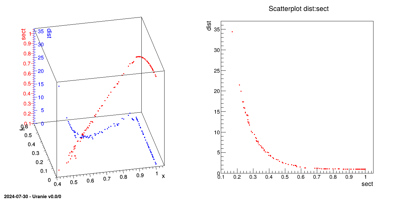
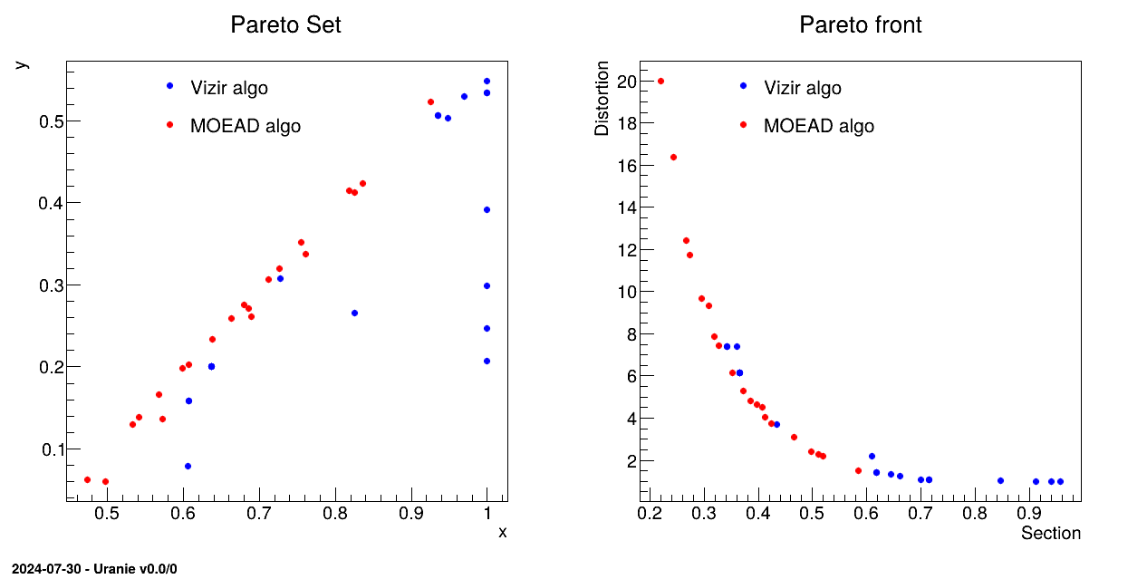
The objective of the macro is to optimize the section and distortion of the hollow bar defined in Section IX.2.2 using the evolutionary solvers, with a reduce number of points to compose the Pareto set/front. This example is comparing both the usual Vizir genetic algorithm and the MOEAD implementation that is meant to be a many-objective criteria algorithm. A short discussion on the many-objective aspect can be found in [metho].
{
#define nbPoints 20
#define total 4*nbPoints
using namespace URANIE::DataServer;
using namespace URANIE::Relauncher;
using namespace URANIE::Reoptimizer;
// variables
TAttribute x("x", 0.0, 1.0),
y("y", 0.0, 1.0),
thick("thick"), // thickness
sect("sect"), // section of the pipe
dist("dist"); // distortion
gROOT->LoadMacro("UserFunctions.C");
// Creating the assessor using the analytical function
TCIntEval code("barAllCost");
code.addInput(&x);
code.addInput(&y);
code.addOutput(&thick);
code.addOutput(§);
code.addOutput(&dist);
// Create a runner
TSequentialRun runner(&code);
runner.startSlave(); // Usual Relauncher construction
int nMax=3000;
if(runner.onMaster())
{
// ==================================================
// ========= Classical Vizir implementation =========
// ==================================================
// Create the TDS
TDataServer tds_viz("vizirDemo", "Vizir parameter dataser");
tds_viz.addAttribute(&x);
tds_viz.addAttribute(&y);
// create the vizir genetic solver
 TVizirGenetic solv_viz;
// Set the size of the population to 150, and a maximum number of evaluation at 15000
solv_viz.setSize(nbPoints,nMax);
// Create the multi-objective constrained optimizer
TVizir2 opt_viz(&tds_viz, &runner, &solv_viz);
// add the objective
opt_viz.addObjective(§); // minimizing the section
opt_viz.addObjective(&dist); // minimizing the distortion
// and the constrains
TGreaterFit positiv(0.4);
opt_viz.addConstraint(&thick,&positiv); //on thickness (thick > 0.4)
opt_viz.solverLoop(); // running the optimization
// ==================================================
// ============== MOEAD implementation ==============
// ==================================================
// Create the TDS
TDataServer tds_moead("vizirDemo", "Vizir parameter dataser");
tds_moead.addAttribute(&x);
tds_moead.addAttribute(&y);
// create the vizir genetic solver
TVizirGenetic solv_moead;
solv_moead.setMoeadDiversity(nbPoints);
solv_moead.setStoppingCriteria(1);
solv_moead.setSize(0, nMax, 200);
// Create the multi-objective constrained optimizer
TVizir2 opt_moead(&tds_moead, &runner, &solv_moead);
// add the objective
opt_moead.addObjective(§); // minimizing the section
opt_moead.addObjective(&dist); // minimizing the distortion
opt_moead.addConstraint(&thick,&positiv); //on thickness (thick > 0.4)
opt_moead.solverLoop(); // running the optimization
// Stop the slave processes
runner.stopSlave();
// Start the graphical part
// Preaparing canvas
TCanvas *fig1 = new TCanvas("fig1","Pareto Zone",5,64,1270,667);
TPad *pad1 = new TPad("pad1","",0,0.03,1,1);
pad1->Draw();
pad1->Divide(2,1); pad1->cd(1);
// extracting data to construct graphs
double viz[total], moead[total+4]; // There is always one more point in moead
tds_viz.getTuple()->extractData(viz, total, "x:y:sect:dist","","column");
tds_moead.getTuple()->extractData(moead, total+4, "x:y:sect:dist","","column");
TGraph *set_viz = new TGraph(nbPoints, &viz[0], &viz[nbPoints]);
TGraph *front_viz = new TGraph(nbPoints, &viz[2*nbPoints], &viz[3*nbPoints]);
set_viz->SetMarkerColor(4); set_viz->SetMarkerStyle(20); set_viz->SetMarkerSize(0.8);
front_viz->SetMarkerColor(4); front_viz->SetMarkerStyle(20); front_viz->SetMarkerSize(0.8);
TGraph *set_moead = new TGraph(nbPoints+1, &moead[0], &moead[nbPoints+1]);
TGraph *front_moead = new TGraph(nbPoints, &moead[2*(nbPoints+1)], &moead[3*(nbPoints+1)]);
set_moead->SetMarkerColor(2); set_moead->SetMarkerStyle(20); set_moead->SetMarkerSize(0.8);
front_moead->SetMarkerColor(2); front_moead->SetMarkerStyle(20); front_moead->SetMarkerSize(0.8);
// Legend
TLegend *leg = new TLegend(0.25, 0.75, 0.55, 0.89);
leg->AddEntry(set_viz,"Vizir algo","p");
leg->AddEntry(set_moead,"MOEAD algo","p");
// Pareto Set
TMultiGraph *set_mg = new TMultiGraph();
set_mg->Add(set_viz); set_mg->Add(set_moead);
set_mg->Draw("aP");
set_mg->SetTitle("Pareto Set"); set_mg->GetXaxis()->SetTitle("x"); set_mg->GetYaxis()->SetTitle("y");
leg->Draw();
gPad->Update();
// Pareto Front
pad1->cd(2);
TMultiGraph *front_mg = new TMultiGraph();
front_mg->Add(front_viz); front_mg->Add(front_moead);
front_mg->Draw("aP");
front_mg->SetTitle("Pareto front"); front_mg->GetXaxis()->SetTitle("Section"); front_mg->GetYaxis()->SetTitle("Distortion");
leg->Draw();
gPad->Update();
}
}
The variables are defined as follow:
// variables
TAttribute x("x", 0.0, 1.0),
y("y", 0.0, 1.0),
thick("thick"), // thickness
sect("sect"), // section of the pipe
dist("dist"); // distortionwhere the first two are the input ones while the last ones are computed using the provided code (as explained in Section IX.2.2). This code is configured through these lines
// Creating the assessor using the analytical function
TCIntEval code("barAllCost");
code.addInput(&x);
code.addInput(&y);
code.addOutput(&thick);
code.addOutput(§);
code.addOutput(&dist);
The usual Relauncher construction is followed, using a TSequentialRun runner. The first solver
is defined in these lines
TVizirGenetic solv_viz;
// Set the size of the population to 150, and a maximum number of evaluation at 15000
solv_viz.setSize(nbPoints,nMax);Combining the runner, solver and dataserver, the master object is created and the objective and constraint are defined. This is done in:
// Create the multi-objective constrained optimizer
TVizir2 opt_viz(&tds_viz, &runner, &solv_viz);
// add the objective
opt_viz.addObjective(§); // minimizing the section
opt_viz.addObjective(&dist); // minimizing the distortion
// and the constrains
TGreaterFit positiv(0.4);
opt_viz.addConstraint(&thick,&positiv); //on thickness (thick > 0.4);
In a second block a new dataserver is created along with a new genetic solver in these lines:
// create the vizir genetic solver
TVizirGenetic solv_moead;
solv_moead.setMoeadDiversity(nbPoints);
solv_moead.setStoppingCriteria(1);
solv_moead.setSize(0, nMax, 200);
The idea here is to use the Moead algorithm whose principle in few words is to split the space into a certain
numbers of direction intervals (set by the argument in the function
setMoeadDiversity). This should provide a Pareto front with a better homogeneity in the
front member distribution (particularly visible here when the size of the requested ensemble is small). The second
method, setStoppingCriteria(1) states that the only stopping criteria available is the
total number of estimation, allowed in the setSize method. Finally, the last function to
be called is the setSize one, with a peculiar first argument here: the size of the pareto
can be chosen but if 0 is put (as done here) the number of elements will be the number of intervals defined
previously plus one (the plus one comes from the fact that the elements are created at the edge of every interval,
so for 20 intervals, there are 21 edges in total).
The rest of the code is creating the plot shown below in which both Pareto set and front are compared.
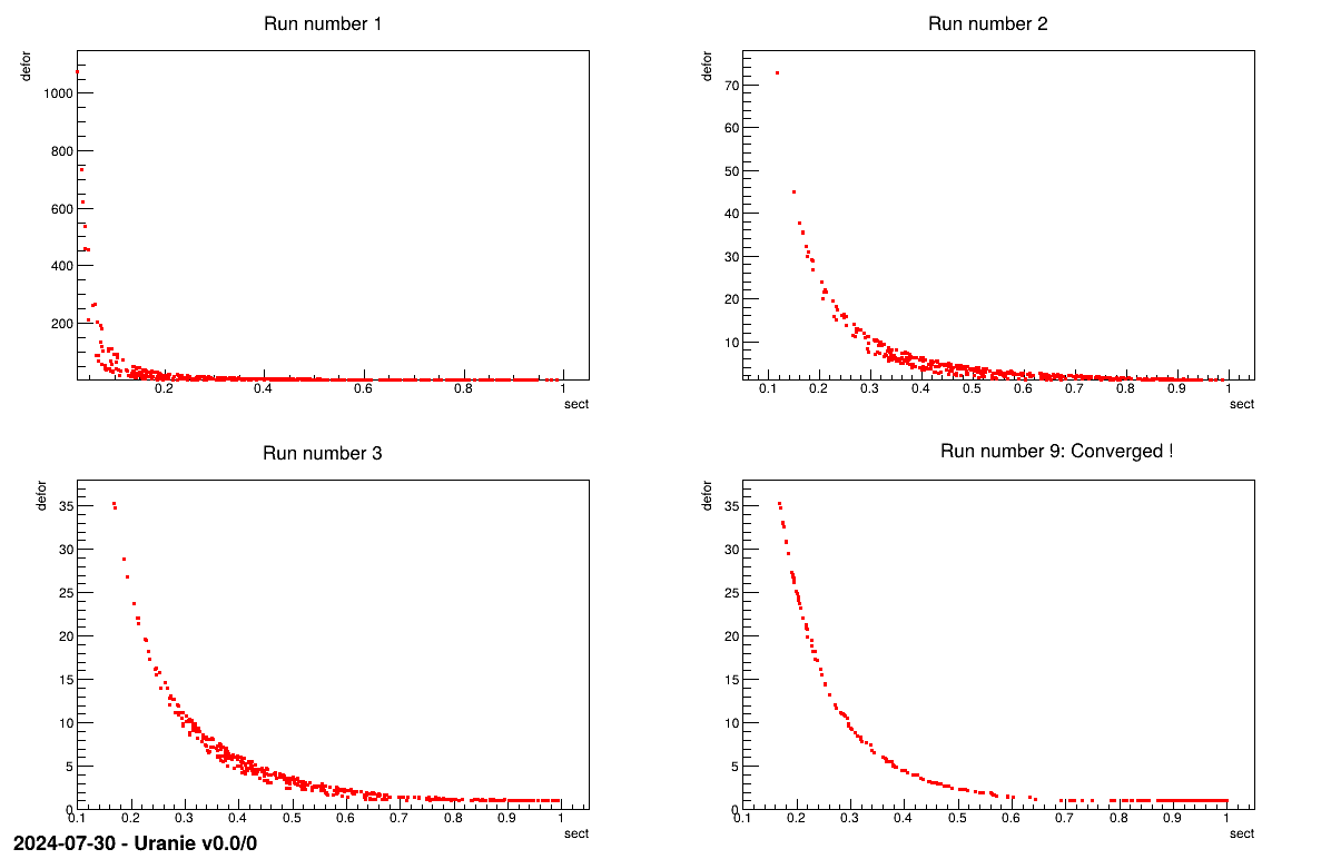
The objective of the macro is to be able to run an evolutionary algorithm (here we are using a genetic one) with a limited number of code estimation and restart it from where it stopped if it has not converged the first time. This is of utmost usefulness when running a resource-consumming code or (/and) when running on a cluster with a limited number of cpu time. The classical hollow bar example defined in Section IX.2.2 is used to obtain a nice Pareto set/front.
#define TOLERANCE 0.001
#define NBmaxEVAL 1200
#define SIZE 500
bool LaunchVizir(int RunNumber, TCanvas *fig1)
{
// variables
TAttribute x("x", 0.0, 1.0),
y("y", 0.0, 1.0),
thick("thick"),
sect("sect"),
def("def");
TCIntEval code("barAllCost");
code.addInput(&x);
code.addInput(&y);
code.addOutput(&thick);
code.addOutput(§);
code.addOutput(&def);
// Create a runner
TSequentialRun runner(&code);
runner.startSlave();
// Output to state whether convergence is reached
bool hasConverged=false;
if(runner.onMaster())
{
// Create the TDS
TDataServer tds("vizirDemo", "Param de l'opt vizir pour la barre");
tds.addAttribute(&x);
tds.addAttribute(&y);
TVizirGenetic solv;
// Name of the file that will contain
string filename="genetic.dump";
std::vector<char> cstr(filename.c_str(), filename.c_str() + filename.size() + 1);
/* Test whether genetic.dump exists. If not, it creates it and returns false, so
that the "else" part is done to start the initialisation of the vizir algorithm. */
if ( solv.setResume(NBmaxEVAL, &cstr[0]))
cout << "Restarting Vizir" << endl;
else solv.setSize(SIZE, NBmaxEVAL);
// Create the multi-objective constrained optimizer
TVizir2 opt(&tds, &runner, &solv);
opt.setTolerance(TOLERANCE);
// add the objective
opt.addObjective(§);
opt.addObjective(&def);
TGreaterFit positiv(0.4);
opt.addConstraint(&thick,&positiv);
/* resolution */
opt.solverLoop();
hasConverged=opt.isConverged();
// Stop the slave processes
runner.stopSlave();
fig1->cd(RunNumber+1);
tds.getTuple()->SetMarkerColor(2);
tds.draw("def:sect");
stringstream tit; tit << "Run number "<<RunNumber+1;
if(hasConverged) tit << ": Converged !";
((TH1F*)gPad->GetPrimitive("__tdshisto__0"))->SetTitle( tit.str().c_str() );
}
return hasConverged;
}
int reoptimizeHollowBarVizirSplitRuns()
{
using namespace URANIE::DataServer;
using namespace URANIE::Relauncher;
using namespace URANIE::Reoptimizer;
gROOT->LoadMacro("UserFunctions.C");
// Delete previous file if it exists
gSystem->Unlink("genetic.dump");
bool finished=false;
int i=0;
TCanvas *fig1 = new TCanvas("fig1","fig1",1200,800);
fig1->Divide(2,2);
while ( ! finished )
{
finished=LaunchVizir(i, fig1);
i++;
}
return 1;
}
The idea is to show how to run this kind of configuration: the function LaunchVizir is
the usual script one can run to get an optimisation with Vizir on the hollow bar problem. The aim is to create a
Pareto set of 500 points (SIZE) but only allowing 1200 estimation (NBmaxEVAL). With this configuration we are sure
that a first round of estimation will not converge, so we will have to restart the optimisation from the point we
stopped. With this regard, the beginning of this function is trivial and the main point to be discussed arises once
the solver is created.
TVizirGenetic solv;
// Name of the file that will contain
string filename="genetic.dump";
std::vector<char> cstr(filename.c_str(), filename.c_str() + filename.size() + 1);
/* Test whether genetic.dump exists. If not, it creates it and returns false, so
that the "else" part is done to start the initialisation of the vizir algorithm. */
if ( solv.setResume(NBmaxEVAL, &cstr[0]))
cout << "Restarting Vizir" << endl;
else solv.setSize(SIZE, NBmaxEVAL);
Clearly here, the interesting part apart, from the definition of the name of the file in which the final state will be kept,
is the first test on the solver, before using the setSize method. A new methods called
setResume is called, with two arguments : the number of elements requested in the Pareto set and the
name of the file in which to save the state or to restart from. This method returns "true" if
genetic.dump is found and "false" if not. In the first case, the code will assume that this file is the
result of a previous run and it will start the optimisation from the its content trying to get all the population
non-dominated (if it's not yet the case). If, on the other hand, no file is found, then the code knows that it would have to
store the results of its process, in a file whose name is the second argument, and because the function returns "false", then
we move to the "else" part, that starts the optimisation.
Apart from this, the rest of the function is doing the optimisation, and plotting the pareto front in a provided canvas. The only new part here is the fact that the solver (its master in fact) is now able to tell whether it has converged or not through the following method
hasConverged=opt.isConverged();this argument being return as the results of the function.
This macro contains another function called reoptimizeHollowBarVizirSplitRuns which plays
the role of the user in front of a ROOT-console. It defines the correct namespace, loads the function file and
destroys previously existing genetic.dump files. From there it runs the
LaunchVizir function as many times as needed (thanks to the boolean returned) as the used
would do, by restarting the macro, even after exiting the ROOT console.
The plot shown below represent the Pareto front every time the genetic algorithm stops (at the fourth run, it finally converges !).
The objective of the macro is to show an example of a two level parallelism program using the Mpi paradigm.
At the top level, an optimization loop parallelizes its evaluations
At low level, each optimizer evaluation are a launcher loop who parallelizes its own sequential evaluations
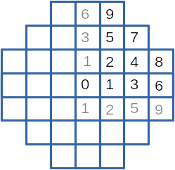
These example is inspired from a zoning problem of a small plant core with square assemblies. However, the physics embeded in it is reduced to none (sorry), and the problem is simplified. With symetries, the core is defined by 10 different assemblies presented on the following figure. For production purpose, only 5 assembly types are allowed, defined by an emission value.
To simplify the problem, some constraints are put :
most assemblies belong to a default zone
other zone is restricted to one assembly (or two for 4 and 5, and for 8 and 9 for symetrical reason)
one zone is imposed with the 8th et 9th external assemblies.
the total of assembly emission is defined.
For each assembly, a reception value is defined depending on the emission from itself and its neighbour's (just 8 neightbours are taken in account, the 4 nearest neighbours and 4 secondary neighbours). The global objective is to minimize the difference between the biggest and the smallest reception value.
Optimisation works on 4 emission values (the fifth value, affected to the external zone, is set, and all values are normalized with the total emission value) and each evaluation loops over the 35 possible arrangements (choose 3 zones from 7). A single evaluation take emission values and the selected zones and return the maximum reception difference.
This macro is splited in 2 files : the first one defines the low level evaluation function and is reused in the next reoptimizer example. It is quite a mock function, and is given to be complete, but is not needed to understand how to implement the two level MPI parallelism
/*
the different zones

6 9
3 5 7
1 2 4 8
0 1 3 6
1 2 5 9

*/

// 4 primary neighbours of a zone
int near1[10][4] = {
  {1,1,1,1}, {0,2,2,3}, {1,1,4,5}, {1,4,5,6}, {2,3,7,8}, // 0-4
  {2,3,7,9}, {3,8,9,10}, {4,5,10,10}, {4,6,10,10}, {5,6,10,10}  // 5-9
};

// 4 secondary neighbours
int near2[10][4] = {
  {2,2,2,2}, {1,1,4,5}, {0,3,3,7}, {2,2,8,9}, {1,5,6,10}, //4
  {1,4,6,10}, {4,5,10,10}, {2,8,9,10}, {3,7,10,10}, {3,7,10,10}  //9
};

// low level evaluation

void lowfun(double *in, double *out)
// evaluate a zoning
{
    double dft;
    double all, min, max, next;
    int p, i, j, id;
    double loc[11], bar[11];

    // init dft
    dft = in[0];
    for (i=0; i<8; i++) loc[i] = dft;
    loc[8] = loc[9] = 0.8;
    loc[10] = 0.;
    // init spec
    for (i=4; i<7; i++) {
        id = (int) in[i];
        loc[id] = in[i-3];
        if (id == 4) loc[5] = in[i-3];
    }
    // normalize
    all = loc[0]/4;
    for (i=1; i<11; i++) all += loc[i];
    for (i=0; i<11; i++) loc[i] *= 10/all;

    // max diff
    i=0;
    next = loc[i];
    for (j=0; j<4; j++) next += loc[near1[i][j]]/8;
    for (j=0; j<4; j++) next += loc[near2[i][j]]/16;
    max = min = next;

    for (i=1; i<10; i++) {
        next = loc[i];
        for (j=0; j<4; j++) next += loc[near1[i][j]]/8;
        for (j=0; j<4; j++) next += loc[near2[i][j]]/16;
        if (next < min) min = next;
        else if (next > max) max = next;
    }

    out[0] = max-min;
    for (i=0; i<10; i++) out[i+1] = loc[i];
}
The lowfun function deals, as expected, with the low level evaluation. In inputs it has the 4 emission
values (default, zone1, zone2, zone3) and 3 indicators defining the zone affected by the extra emission value. It
returns the maximal difference between two zone reception values and the 9 normalized emission values (informative
data). Two arrays are used to define the neighbourhood
With the second file, the two level MPI parallelism is defined.
using namespace URANIE::DataServer;
using namespace URANIE::Relauncher;
using namespace URANIE::Reoptimizer;
using namespace URANIE::MpiRelauncher;

#include "reoptimizeZoneCore.C"

void tds_resume(TDataServer *tds, TAttribute **att, double *res)
{
    TList leaves;
    TLeaf *leaf;
    int i, j, k, siz;
    double obj, cur;
    std::vector<double> tmp;

    siz = tds->getTuple()->GetEntries();

    // init
    for (i=0; att[i]; i++) {
        leaves.Add(tds->GetTuple()->GetLeaf(att[i]->GetName()));
    }
    tmp.resize(i);

    // search min
    tds->GetTuple()->GetEntry(0);
    obj = ((TLeaf *) leaves.At(0))->GetValue(0);
    k = 0;
    for (i=1; i<siz; i++) {
        tds->GetTuple()->GetEntry(i);
        cur = ((TLeaf *) leaves.At(0))->GetValue(0);
        if (cur < obj) {
            obj = cur;
            k = i;
        }
    }

    // get all results
    TIter nextl(&leaves);
    tds->GetTuple()->GetEntry(k);
    for (j=0; (leaf = (TLeaf *) nextl() ); j++) {
        res[j] = leaf->GetValue(0);
    }

}

int doefun(double *in, double *out)
{
    double z0, z1, z2, z3;
    int i;

    // const
    z0 = in[0];
    z1 = in[1];
    z2 = in[2];
    z3 = in[3];

    // inputs
    TAttribute zon0("zon0", 0., 1.);
    TAttribute zon1("zon1", 0., 1.);
    TAttribute zon2("zon2", 0., 1.);
    TAttribute zon3("zon3", 0., 1.);
    TAttribute a1("a1");
    TAttribute a2("a2");
    TAttribute a3("a3");
    TAttribute *funi[] = { &zon0, &zon1, &zon2, &zon3, &a1, &a2, &a3, NULL};
    //output
    TAttribute diff("diff");
    TAttribute v0("v0");
    TAttribute v1("v1");
    TAttribute v2("v2");
    TAttribute v3("v3");
    TAttribute v4("v4");
    TAttribute v5("v5");
    TAttribute v6("v6");
    TAttribute v7("v7");
    TAttribute v8("v8");
    TAttribute v9("v9");
    TAttribute *funo[] = {
        &diff, &v0, &v1, &v2, &v3, &v4, &v5, &v6, &v7, &v8, &v9, NULL
    };

    // funlow
    TCJitEval lfun(lowfun);
    for (i=0; funi[i]; i++) lfun.addInput(funi[i]);
    for (i=0; funo[i]; i++) lfun.addOutput(funo[i]);

    // runner
    // TSequentialRun run(&lfun);
    TSubMpiRun run(&lfun);
    run.startSlave();
    if (run.onMaster()) {
        TDataServer tds("doe", "tds4doe");
        tds.keepFinalTuple(kFALSE);
        for (i=4; i<7; i++) tds.addAttribute(funi[i]);
        tds.fileDataRead("reoptimizeZoneDoe.dat", kFALSE, kTRUE, "quiet");

        TLauncher2 launch(&tds, &run);
        launch.addConstantValue(&zon0, z0);
        launch.addConstantValue(&zon1, z1);
        launch.addConstantValue(&zon2, z2);
        launch.addConstantValue(&zon3, z3);
        // run doe
        launch.solverLoop();

        //get critere
        tds_resume(&tds, funo, out);

        run.stopSlave();
    }
    return 1;
}

void reoptimizeZoneBiSubMpi()
{
    //ROOT::EnableThreadSafety();
    int i;

    // inputs
    TAttribute z1("zone1", 0., 1.);
    TAttribute z2("zone2", 0., 1.);
    TAttribute z3("zone3", 0., 1.);
    TAttribute z4("zone4", 0., 1.);
    TAttribute *zo[] = { &z1, &z2, &z3, &z4, NULL };

    // outputs
    TAttribute diff("diff");
    TAttribute v0("v0");
    TAttribute v1("v1");
    TAttribute v2("v2");
    TAttribute v3("v3");
    TAttribute v4("v4");
    TAttribute v5("v5");
    TAttribute v6("v6");
    TAttribute v7("v7");
    TAttribute v8("v8");
    TAttribute v9("v9");
    TAttribute *out[] = {
        &diff, &v0, &v1, &v2, &v3, &v4, &v5, &v6, &v7, &v8, &v9, NULL
    };

    // fonction
    TCJitEval fun(doefun);
    for (i=0; zo[i]; i++) fun.addInput(zo[i]);
    for (i=0; out[i]; i++) fun.addOutput(out[i]);
    fun.setMpi();

    // runner
    //TThreadedRun runner(&fun,8);
    //TSequentialRun runner(&fun);
    TBiMpiRun runner(&fun, 3);
    runner.startSlave();
    if (runner.onMaster()) {
        TDataServer tds("tdsvzr", "tds4optim");
        fun.addAllInputs(&tds);

        //
        TVizirGenetic gene;
        gene.setSize(300, 200000, 100);
        //TVizirIsland viz(&tds, &runner, &gene);
        TVizir2 viz(&tds, &runner, &gene);
        //viz.setTolerance(0.00001);
        viz.addObjective(&diff);

        viz.solverLoop();

        runner.stopSlave();
        tds.exportData("__coeur__.dat");
    }
}
This script is structured with 3 functions :
function
tds_resumeis used by the intermediate function. It receives theTDataServerfilled, loops on its items and returns an synthetic value. In our case, the minimum value of the reception difference, and the 9 normalized emission valuesfunction
doefunis the intermediate evaluation function. It runs the design of experiments containing all 35 possible arrangements and extract the best one. It receives the 4 emission values and used them to complete theTDataServerusing theaddConstantValuemethod.function
reoptimizeZoningBiSubMpiis the top level function who solve the zoning problem
TBiMpiRun and TSubMpiRun are used to allocate cpus between
intermediate and low level. TBiMpiRun is used in reoptimizeZoningBiSubMpi (top)
with an integer argument specifying the number of CPUs dedicated to each intermediate level. In our case (3), with
16 resources request to MPI, they are divided in 5 groups of 3 CPUs, and one CPU is left for the top level master
(take care that the number of CPUs requested matches group size (16 % 3 == 1)). The top level Master sees 5
resources for his evaluations. TSubMpiRun is used in doefun function and gives
access to the 3 own resources reserved in top level function.
Running the script is done as usual with MPI :
mpirun -n 16 root -l -b -q reoptimizeZoningBiSubMpi.C
At the begining of reoptimizeZoningBiSubMpi function there is a call to
ROOT::EnableThreadSafety. It is unusefull in this case, but if we parallelize with threads instead
of MPI. If you want to use both threads and MPI, it is recommended to use MPI at top level.
The objective of the macro is to give another example of a two level parallelism program using MPI paradigm. In the former example MPI function call is implicit using Uranie facilities. In this one, explicit calls to MPI functions is done. It's presented to illustrate the case when the user evaluation fonction is an MPI function.
It takes the former example of zoning problem and adapts it. The intermediate level does not use a
TLauncher2 to run all different arrangements, but encodes it. Each Mpi ressources evaluates different
possible arrangements keeping its best one, and Mpi reduce these results to the final result.
The low level evaluation function is the same than in previous example and is not shown again.
using namespace URANIE::DataServer;
using namespace URANIE::Relauncher;
using namespace URANIE::Reoptimizer;
using namespace URANIE::MpiRelauncher;

#include "reoptimizeZoneCore.C"
#include "reoptimizeZoneDoe.h"

struct mpiret {
    double val;
    int id;
};

int doefun(double*, double*);

void reoptimizeZoneBiFunMpi()
{
    ROOT::EnableThreadSafety();
    int i;

    // inputs
    TAttribute z1("zone1", 0., 1.);
    TAttribute z2("zone2", 0., 1.);
    TAttribute z3("zone3", 0., 1.);
    TAttribute z4("zone4", 0., 1.);
    TAttribute *zo[] = { &z1, &z2, &z3, &z4, NULL };

    // outputs
    TAttribute diff("diff");
    TAttribute v0("v0");
    TAttribute v1("v1");
    TAttribute v2("v2");
    TAttribute v3("v3");
    TAttribute v4("v4");
    TAttribute v5("v5");
    TAttribute v6("v6");
    TAttribute v7("v7");
    TAttribute v8("v8");
    TAttribute v9("v9");
    TAttribute *out[] = {
        &diff, &v0, &v1, &v2, &v3, &v4, &v5, &v6, &v7, &v8, &v9, NULL
    };

    // fonction
    TCJitEval fun(doefun);
    for (i=0; zo[i]; i++) fun.addInput(zo[i]);
    for (i=0; out[i]; i++) fun.addOutput(out[i]);

    // runner
    //TThreadedRun runner(&fun,8);
    //TSequentialRun runner(&fun);
    TBiMpiRun runner(&fun, 3);
    runner.startSlave();
    if (runner.onMaster()) {
        TDataServer tds("tdsvzr", "tds4optim");
        fun.addAllInputs(&tds);

        //
        TVizirGenetic gene;
        gene.setSize(300, 200000, 100);
        //TVizirIsland viz(&tds, &runner, &gene);
        TVizir2 viz(&tds, &runner, &gene);
        //viz.setTolerance(0.00001);
        viz.addObjective(&diff);

        viz.solverLoop();

        runner.stopSlave();
        tds.exportData("__coeurM__.dat");
    }
}

int doefun(double *in, double *out)
{
    int i, id, size, fid, tag;
    MPI_Comm comm;
    double z[7], one[11], two[11];
    double *cur, *mem, *swp;
    struct mpiret ret, res;

    comm = URANIE::MpiRelauncher::TBiMpiRun::getCalculMpiComm();
    MPI_Comm_rank(comm, &id);
    MPI_Comm_size(comm, &size);

    // const
    z[0] = in[0];
    z[1] = in[1];
    z[2] = in[2];
    z[3] = in[3];

    // local
    mem = one;
    cur = two;
    i = id;
    z[4] = doe[i][0];
    z[5] = doe[i][1];
    z[6] = doe[i][2];
    lowfun(z, mem);
    for (i = id+size; i<DOESIZE; i+=size) {
        z[4] = doe[i][0];
        z[5] = doe[i][1];
        z[6] = doe[i][2];
        lowfun(z, cur);
        if (cur[0] < mem[0]) {
            swp = mem;
            mem = cur;
            cur = swp;
        }
    }

    // global
    /* where is min */
    ret.val = mem[0];
    ret.id = id;
    MPI_Allreduce(&ret, &res, 1, MPI_DOUBLE_INT, MPI_MINLOC, comm);

    /* get min extra datas */
    if (res.id != 0) {
        if (id == res.id) {
            MPI_Send(mem, 11, MPI_DOUBLE, 0, 0, comm);
        }
        else if (id == 0) {
            MPI_Recv(out, 11, MPI_DOUBLE, res.id, 0, comm, MPI_STATUS_IGNORE);
        }
    }
    else {
        for (i=0; i<11; i++) out[i] = mem[i];
    }
    return 1;
}
The top level function (reoptimizeZoneBiFunMpi) does not change from the previous example and defines a
TBiMpiRun instances.
The evaluation MPI fonction (doefun) is totaly different. It uses the class method
URANIE::MpiRelauncher::TBiMpiRun::getCalculMpiComm to get the MPI Communicator object
(MPI_Comm) dedicated to the calcul ressources. With it, different call to MPI functions can be done :
MPI_Comm_rank and MPI_Comm_size to get the context ; MPI_Allreduce,
MPI_Send and MPI_Recv to communicate between calculs ressources.
Note that the evaluation function is predeclared and defined after the top level function. It is a trick for cling (the
ROOT jit compiler) to know the MPI function : when it compiles, it sees the TBiMpiRun
before, and loads MPI librairies. With a real MPI user code, which needs a library, cling cannot be used. User needs
extra works to make it run (build a standalone program or a ROOT compatible library), but the principle presented
before is suitable.
You may run this script the same way as the precedent example, with the same constraint on the ressource number. Also
note that this version is really faster than the previous one, avoiding creation and manipulation of a
TDataServer.
| |  | |
| XIV.8. Macros Relauncher |  | XIV.10. Macros MetaModelOptim |