Documentation / User's manual in Python :

III.3. Description of a correlation

III.3. Description of a correlation
	Chapter III. The Sampler module

III.3. Description of a correlation

We will describe in this section how to precise in Uranie the necessary information to take into account the correlations between variables. There are two ways to specify this: setting the correlation coefficient by hand or couple the two considered attributes with a copula. Both methods are described below.

III.3.1. Imposing the correlation coefficients

It is possible to set the correlation coefficient by hand, using the setUserCorrelation method of both TSampling and TBasicSampling.

xunif = DataServer.TUniformDistribution("x1", 3., 4.)  
xnorm = DataServer.TNormalDistribution("x2", 0.5, 1.5)   

tds = DataServer.TDataServer("tdsSampling", "Demonstration Sampling")
tds.addAttribute(xunif)
tds.addAttribute(xnorm)

# Generate the sampling from the TDataServer object
sampling = Sampler.TSampling(tds, "lhs", 1000)
sampling.setUserCorrelation(xunif, xnorm, 0.90)    
sampling.generateSample()   
tds.Draw("x2:x1", "", "")

Specification of a correlation

	Generating a uniform random variable in [3., 4.]
	Generating a gaussian random variable with 0.5 as mean value 1.5 as standard deviation.
	Specification of correlation of 0.90 between the two attributes `xunif` and `xnorm`.
	Generate the sample by calling the `generateSample` method in `TSampling` (respectively the `generateCorrSample` method in `TBasicSampling`).

The coefficient provided is changing the correlation between the two considered attributes (for a more general discussion on this, see [metho]). As an example, Figure III.4 and Figure III.5 show the design-of-experiments created with the TSampling class, using a normal and uniform distribution, using three different correlation coefficient values: 0, 0.45 and 0.9. The first one is showing the obtained 2D plan and their corresponding projections, while the second one is showing the same information but displaying their rank instead of their values (this is further discussed in [metho]).

Figure III.4. Tufte plot of the design-of-experiments created using a normal and uniform distribution, with a LHS method with three correlation coefficient: 0, 0.45 and 0.9

Tufte plot of the design-of-experiments created using a normal and uniform distribution, with a LHS method with three correlation coefficient: 0, 0.45 and 0.9

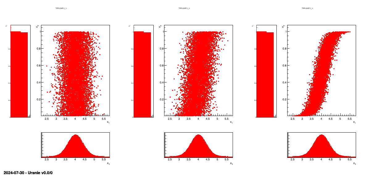Figure III.5. Tufte plot of the rank of the design-of-experiments created using a normal and uniform distribution, with a LHS method with three correlation coefficient: 0, 0.45 and 0.9

Tufte plot of the rank of the design-of-experiments created using a normal and uniform distribution, with a LHS method with three correlation coefficient: 0, 0.45 and 0.9

Instead of provided one-by-one the correlation factors, one can provide the correlation matrix using the setCorrelationMatrix method of both TSampling and TBasicSampling. This method ask for a TMatrixD input and it will check that:

the dimension is correct : .
the coefficient are all in the range
the diagonal term are exactly at one (if not it sets them to this value).

III.3.1.1. Case of singular correlation matrix

In the case where the correlation matrix injected (at once or component by component) happen to be singular, the default method used to correlate variables will failed and complains in this way (taking the TBasicSampling as an example):

<URANIE::ERROR> 
<URANIE::ERROR> *** URANIE ERROR ***
<URANIE::ERROR> *** File[${SOURCEDIR}/meTIER/sampler/souRCE/TBasicSampling.cxx] Line[427]
<URANIE::ERROR> TBasicSampling::generateCorrSample: the cholesky decomposition of the user correlation matrix is not good.
<URANIE::ERROR>  Maybe you can try with SVD decomposition.
<URANIE::ERROR> *** END of URANIE ERROR ***
<URANIE::ERROR>

There is a workaround, provided by Uranie and heavily discussed in [metho]. The idea in a nutshell is to remplace the Cholesky operation by a SVD one, to decompose the target correlation matrix. This can be done adding "svd" in the Option_t *option field of either the constructor of the class or the generator method call. Here is an example for the TBasicSampling class:

tbs = Sampler.TBasicSampling(tds, "lhs;svd", 100)  # example at constructor
# .. or ..
tbs.generateCorrSample("svd")  # example with generator function call

Here comes its equivalent piece of code for the TSampling class:

ts = Sampler.TSampling(tds, "lhs;svd", 100)  # example at constructor
# .. or ..
ts.generateSample("svd")  # example with generator function call

In both cases, the use of this workaround should print this message to warn you about this.

<URANIE::INFO> 
<URANIE::INFO> *** URANIE INFORMATION ***
<URANIE::INFO> *** File[${SOURCEDIR}/meTIER/sampler/souRCE/TBasicSampling.cxx] Line[371]
<URANIE::INFO> TBasicSampling::generateCorrSample: you've asked to use SVD instead of Cholesky to decompose the correlation matrix. 
<URANIE::INFO> *** END of URANIE INFORMATION ***
<URANIE::INFO>

An example of how to use this in real condition (with a proper singular correlation matrix) is shown in Section XIV.4.14.

III.3.2. The copula classes

Instead of using samplers with correlation matrix in the case of intricate variables, one can use classes relying on Copula, in order to describe the dependencies. These classes inherit from the TCopula class successively through the TSamplerStochastic and the TSampler classes. The idea of a copula is to define the interaction of variables using a parametric-function that can allow a broader range of entanglement than only using a correlation matrix (various shapes can be done). There are two kinds of copulas provided in the Uranie platform:

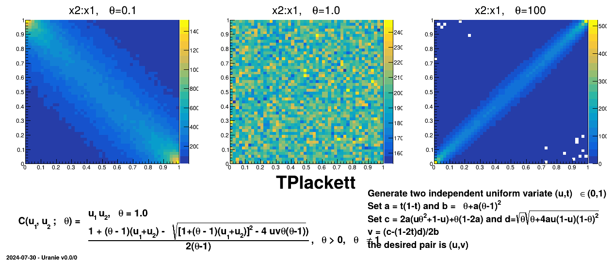
TArchimedian with 4 pre-defined parametrisation: Ali-Mikhail-Haq (TAMHCopula), Clayton (TClaytonCopula), Frank (TFrankCopula) and Plackett (TPlackettCopula). These copulas, which depend only on the input variables and a parameter , are shown from Figure III.6 to Figure III.9 for different values along with the formula of the corresponding parametric function.
TElliptical: it is a class to interface the TGaussian copula method.

Figure III.6. Example of sampling done with half million points and two uniform attributes (from 0 to 1), using AMH copula and varying the parameter value.

Example of sampling done with half million points and two uniform attributes (from 0 to 1), using AMH copula and varying the parameter value.

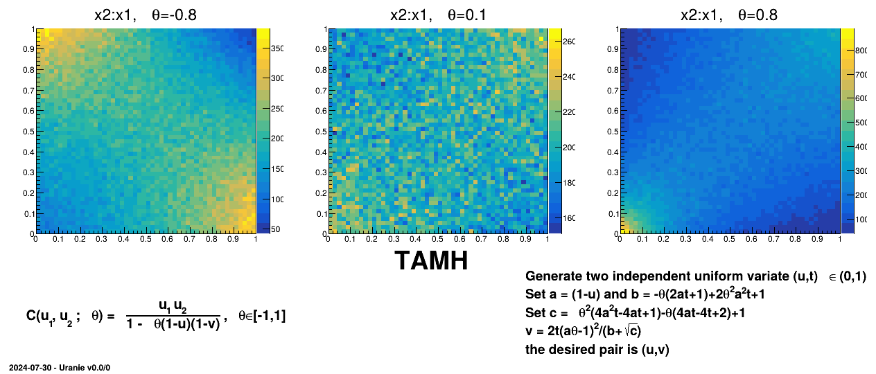Figure III.7. Example of sampling done with half million points and two uniform attributes (from 0 to 1), using Clayton copula and varying the parameter value.

Example of sampling done with half million points and two uniform attributes (from 0 to 1), using Clayton copula and varying the parameter value.

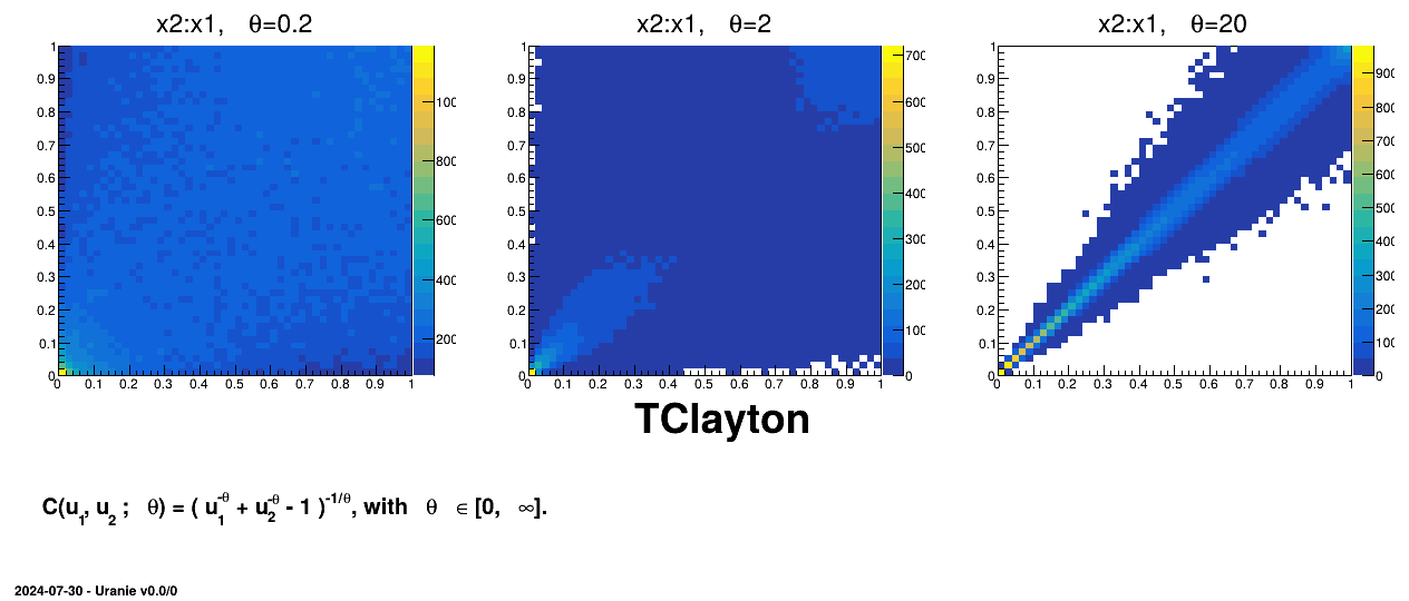Figure III.8. Example of sampling done with half million points and two uniform attributes (from 0 to 1), using Frank copula and varying the parameter value.

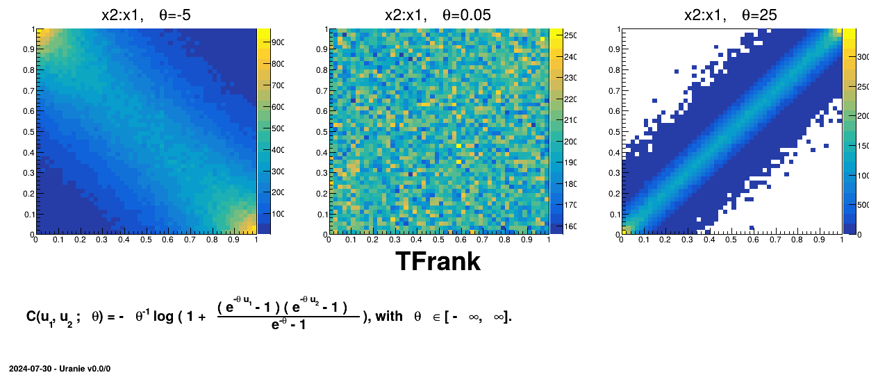Example of sampling done with half million points and two uniform attributes (from 0 to 1), using Frank copula and varying the parameter value.

Figure III.9. Example of sampling done with half million points and two uniform attributes (from 0 to 1), using Plackett copula and varying the parameter value.

Example of sampling done with half million points and two uniform attributes (from 0 to 1), using Plackett copula and varying the parameter value.

The following example shows how to create a copula and to use it in order to get a correlated sample.

xunif = DataServer.TUniformDistribution("x1", 3., 4.)
xnorm = DataServer.TNormalDistribution("x2", 0.5, 1.5)

tds = DataServer.TDataServer("tdsSampling", "Demonstration Sampling")
tds.addAttribute(xunif)
tds.addAttribute(xnorm)

# Generate the sampling from the TDataServer object
tamh = Sampler.TAMHCopula(tds, 0.75, 1000)
tamh.generateSample()
tds.Draw("x2:x1", "", "colZ")


III.2. The Stochastic methods		III.4. QMC method