

Documentation
/ User's manual in Python
: 
| VI.6. Fourier-based methods | ||
|---|---|---|
 | Chapter VI. The Sensitivity module |  |
This section is a short excerpt of [metho]
The Fourier Amplitude Sensitivity Test (FAST) [MCRAE198215, SALTELLI1998445] is a
procedure that provides a way to estimate the expected value and variance of the output variable of a model, along
with the contribution of the input factors to this variance. An advantage of it, is that the evaluation of
sensitivity can be carried out independently for each factor using just a set of runs because all the terms in a
Fourier expansion are mutually orthogonal. The main idea behind this procedure is to transform the  -dimensional integration into a
single-dimension one, by using the transformation
-dimensional integration into a
single-dimension one, by using the transformation
where ideally,  is a set of angular frequencies said to be incommensurate (meaning that no frequency can be
obtained by linear combination of the other ones when using integer coefficients) and
is a set of angular frequencies said to be incommensurate (meaning that no frequency can be
obtained by linear combination of the other ones when using integer coefficients) and  is a transformation function chosen in order to ensure
that the variable is sampled accordingly with the probability density function of
is a transformation function chosen in order to ensure
that the variable is sampled accordingly with the probability density function of  (meaning that they are all uniformly distributed in their
respective volume definition).
(meaning that they are all uniformly distributed in their
respective volume definition).
The first order coefficient is then obtained by estimating the variance for a fundamental  and its harmonics. The important point to
notice, for a real computation, is the limitation of the sum that, in the previous equation, runs up to infinity. A
truncation is done by imposing a cut-off with a factor
and its harmonics. The important point to
notice, for a real computation, is the limitation of the sum that, in the previous equation, runs up to infinity. A
truncation is done by imposing a cut-off with a factor  called the interference factor (whose default
value in Uranie is set to 6).
called the interference factor (whose default
value in Uranie is set to 6).
The Random Balance Design (RBD) [Tarantola2006717] method selects
 design points over a curve
in the input space. The input space is explored here using the same frequency
design points over a curve
in the input space. The input space is explored here using the same frequency  . However the curve is not space-filling, therefore, we
take random permutations of the coordinates of such points, to generate a set of scrambled points that cover the
input space. The model is then evaluated at each design point. Subsequently, the model outputs are re-ordered such
that the design points are in increasing order with respect to factor .
. However the curve is not space-filling, therefore, we
take random permutations of the coordinates of such points, to generate a set of scrambled points that cover the
input space. The model is then evaluated at each design point. Subsequently, the model outputs are re-ordered such
that the design points are in increasing order with respect to factor .
Thanks
to the use of permutations, the total cost is of the order of assessments instead of the order of  for the FAST one.
Both TFAST and TRBD can be constructed either
from an external code or from a function. In the implementation done within Uranie there are several
modifiable parameters that can be considered before starting an analysis using the FAST method:
The transformation function
chosen among the following list:
Cukier:
SaltelliA:

SaltelliB:

In this list,
 is the nominal value of the factor ,
  denotes the endpoints that define the estimated range of uncertainty of ,
  is a random phase shift taken value in
  and
and
 evolves in
  .
.
The interference factor:
can be changed as well.
The frequencies: by providing a vector, it is possible to set a default at the frequencies' value used instead of having them determined by a specific algorithm to avoid, as best as possible, the interference.
The only common parameter changeable for both methods (and directly in the construction) is the number of
samples. Once the object is constructed, running the computeIndexes
will compute the sensitivity indices and the usual drawing methods will allow to retrieve and represent the results,
as already explained for other methods.
Warning
If the Fourier-based object is constructed to run a function, the output used for the estimation will be the first output provided by the function, unless the sixth argument of the constructor is filled.
In Uranie, computing sensitivity with the FAST method is dealt with the eponymous class TFast
which inherits from the TSensitivity class.
This class handles all the steps to compute the Sobol indices:
- generating the deterministic sample;
- running the code or the analytic function to get the response on the sample;
- computing the first order index for each input variable.
The example script below uses the TFast class to compute and display Sobol sensitivity indices:
"""
Example of fast estimation of sensitivity indices
"""
from rootlogon import ROOT, DataServer, Sensitivity
ROOT.gROOT.LoadMacro("UserFunctions.C")
# Define the DataServer
tds = DataServer.TDataServer("tdsflowreate", "DataBase flowreate")
tds.addAttribute(DataServer.TUniformDistribution("rw", 0.05, 0.15))
tds.addAttribute(DataServer.TUniformDistribution("r", 100.0, 50000.0))
tds.addAttribute(DataServer.TUniformDistribution("tu", 63070.0, 115600.0))
tds.addAttribute(DataServer.TUniformDistribution("tl", 63.1, 116.0))
tds.addAttribute(DataServer.TUniformDistribution("hu", 990.0, 1110.0))
tds.addAttribute(DataServer.TUniformDistribution("hl", 700.0, 820.0))
tds.addAttribute(DataServer.TUniformDistribution("l", 1120.0, 1680.0))
tds.addAttribute(DataServer.TUniformDistribution("kw", 9855.0, 12045.0))
# Size of a sampling.
nS = 500
# Graph
tfast = Sensitivity.TFast(tds, "flowrateModel", nS)
tfast.computeIndexes("graph")
cc = ROOT.TCanvas("canhist", "histgramme", 1)
tfast.drawIndexes("Flowrate", "", "nonewcanv, hist, first")
ccc = ROOT.TCanvas("canpie", "TPie", 1)
apad = ROOT.TPad("apad", "apad", 0, 0.03, 1, 1)
apad.Draw()
apad.cd()
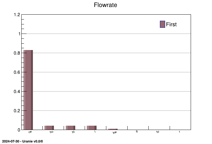
tfast.drawIndexes("Flowrate", "", "nonewcanv, pie, first")
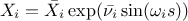
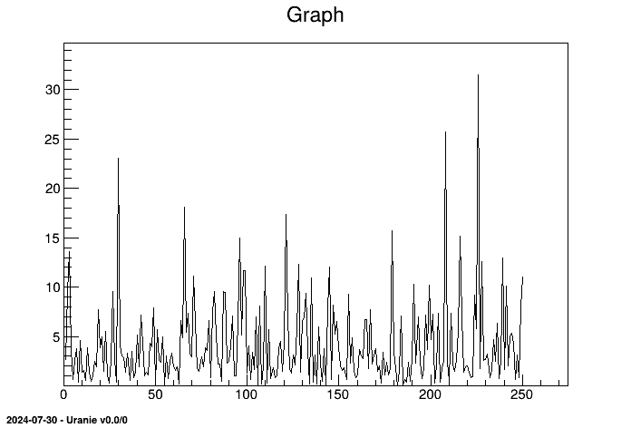
The figures resulting from this script are shown below, the first shows the frequencies:
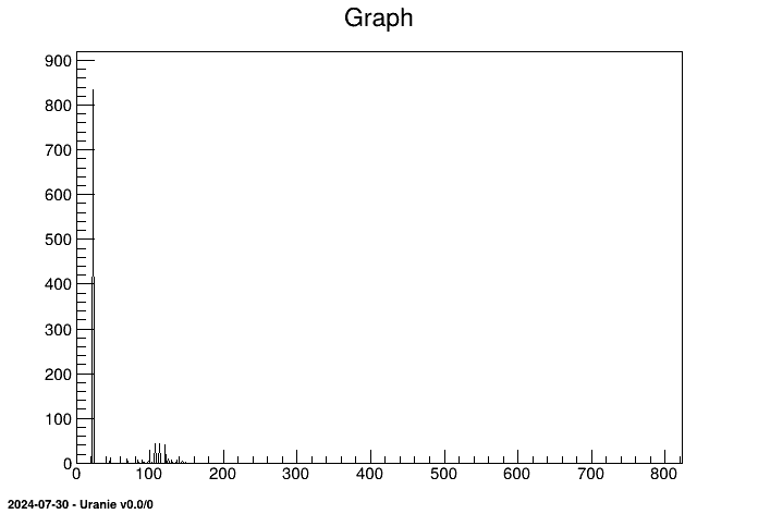
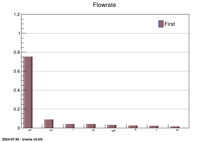
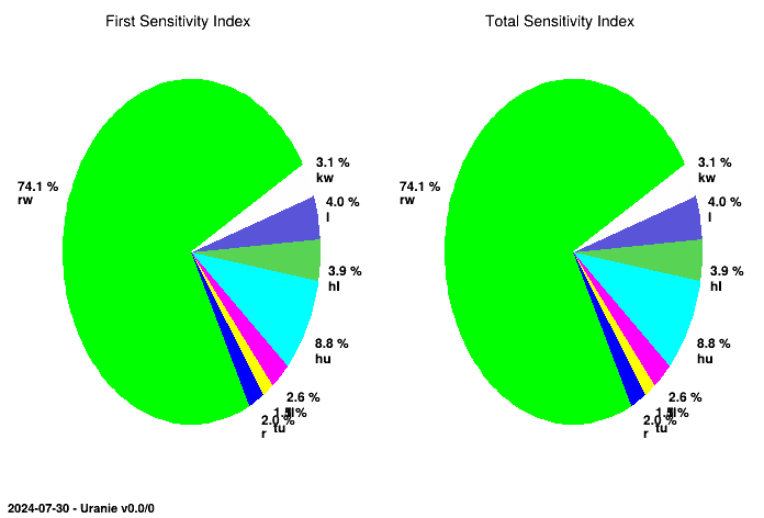
The two figures below display the sensitivity indices in a histogram and in a pie chart:
First, define the uncertain parameters and add them to a TDataServer object:
# Define the DataServer
tds = DataServer.TDataServer("tdsflowreate", "DataBase flowreate")
tds.addAttribute(DataServer.TUniformDistribution("rw", 0.05, 0.15))
tds.addAttribute(DataServer.TUniformDistribution("r", 100.0, 50000.0))
tds.addAttribute(DataServer.TUniformDistribution("tu", 63070.0, 115600.0))
tds.addAttribute(DataServer.TUniformDistribution("tl", 63.1, 116.0))
tds.addAttribute(DataServer.TUniformDistribution("hu", 990.0, 1110.0))
tds.addAttribute(DataServer.TUniformDistribution("hl", 700.0, 820.0))
tds.addAttribute(DataServer.TUniformDistribution("l", 1120.0, 1680.0))
tds.addAttribute(DataServer.TUniformDistribution("kw", 9855.0, 12045.0))
There are three different constructors to build a TFast
object, each corresponding to a different problem:
- the model is an analytic function run by Uranie,
- the model is a code run by Uranie.
- the model is either a function or a code and the problem is specified through a Relauncher architecture.
The constructor prototype used with an analytic function is:
# Create a TFast object with an analytic function
TFast(tds, fcn, inp, out, ns)  # fcn is a function pointer
TFast(tds, fcn, ns, inp = "", out = "", option = "")  # fcn is a string
This constructor takes five arguments:
- a pointer to a
TDataServerobject, - a pointer to an analytic function (either a
voidor aconst charthat represents the function's name when it has been loaded in ROOT's memory), - an integer to specify the number of simulations, its default value is 100,
- a string to specify the names of the input factors separated by ':' (ex. "rw:r:tu:tl:hu:hl:l:kw"), its default value might be the empty string "",
- a string to specify the names of the output variables of the model, its default value might be the empty string "".
Here is an example of how to use the constructor with an analytic function:
ns = 50
tfast = Sensitivity.TFast(tds, "flowrateModel", ns, "rw:r:tu:tl:hu:hl:l:kw", "flowrateModel")The constructor prototype used with a code is:
# Create a TFast object with a code
TFast(tds, fcode,  ns, option = "")
This constructor takes three arguments:
- a pointer to a
TDataServerobject, - a pointer to a
TCode, - an integer to specify the number of simulations.
Here is an example of the use of this constructor on the flowrate case:
# The reference input file
sJDDReference = "flowrate_input_with_keys.in"

# Set the reference input file and the key for each input attributes
tds.getAttribute("rw").setFileKey(sJDDReference, "Rw")
tds.getAttribute("r").setFileKey(sJDDReference, "R")
tds.getAttribute("tu").setFileKey(sJDDReference, "Tu")
tds.getAttribute("tl").setFileKey(sJDDReference, "Tl")
tds.getAttribute("hu").setFileKey(sJDDReference, "Hu")
tds.getAttribute("hl").setFileKey(sJDDReference, "Hl")
tds.getAttribute("l").setFileKey(sJDDReference, "L")
tds.getAttribute("kw").setFileKey(sJDDReference, "Kw")

# The output file of the code
fout = Launcher.TOutputFileRow("_output_flowrate_withRow_.dat")
# The attribute in the output file
fout.addAttribute(DataServer.TAttribute("yhat"))

# Instanciation de mon code
mycode = Launcher.TCode(tds, "flowrate -s -k")
# Adding the outputfile to the tcode object
mycode.addOutputFile(fout)

# Size of a sampling.
nS = 50
tfastC = Sensitivity.TFast(tds, mycode, nS) The constructor prototype used with a runner is:
# Create a TFast object with a runner
TFast(tds, run, ns, option = "")
This constructor takes three arguments:
- a pointer to a
TDataServerobject, - a pointer to a
TRun, - an integer to specify the number of simulations.
Here is an example of the use of this constructor on the flowrate code in a sequential mode:
# The input file
infile = Relauncher.TKeyScript("flowrate_input_with_keys.in")
# provide the input and their key
infile.addInput(tds.getAttribute("rw"), "Rw")
infile.addInput(tds.getAttribute("r"), "R")
infile.addInput(tds.getAttribute("tu"), "Tu")
infile.addInput(tds.getAttribute("tl"), "Tl")
infile.addInput(tds.getAttribute("hu"), "Hu")
infile.addInput(tds.getAttribute("hl"), "Hl")
infile.addInput(tds.getAttribute("l"), "L")
infile.addInput(tds.getAttribute("kw"), "Kw")

yhat = DataServer.TAttribute("yhat")
# The output file of the code
outfile = Relauncher.TKeyResult("_output_flowrate_withKey_.dat")
# The attribute in the output file
outfile.addOutput(yhat, "yhat")

# Instanciation de mon code
code = Relauncher.TCodeEval("flowrate -s -k")
# Adding the intput/output file to the code
code.addInputFile(infile)
code.addOutputFile(outfile)

run = Relauncher.TSequentialRun(code)
run.startSlave()
if run.onMaster():

    nS = 50
    tfastR = Sensitivity.TFast(tds, run, nS)
    # ...
To generate the FAST sample, use the generateSample method:
tfast.generateSample()Then, the sample generated can be exported in a file and used outside of Uranie to compute the simulations associated.
To compute the indices, run the method computeIndexes:
tfast.computeIndexes() Note that this method is all inclusive: it constructs the sample, launches the simulations and computes the indices. If the "graph" option is provided, a graph of frequency will be drawn, as the one shown in Figure VI.7
To display graphically the coefficients, use the method drawIndexes:
drawIndexes(sTitre, select, option)The method needs:
- a
TStringcontaining the title of the figure, - a string containing a selection (empty if no selection),
- a string containing the options of the graphics separated by commas.
Some of the options available are:
- "nonewcanv": to not create a new canvas,
- "pie": to display a pie chart,
- "hist": to display a histogram,
- "first": to display the indices of the first order (with "hist" only),
In our example the use of this method is:
cc = ROOT.TCanvas("canhist", "histgramme")
tfast.drawIndexes("Flowrate", "", "nonewcanv,hist,first")
cc.Print("appliUranieFlowrateFAST100Histogram.png")

ccc = ROOT.TCanvas("canpie", "TPie")
tfast.drawIndexes("Flowrate", "", "nonewcanv,pie")
ccc.Print("appliUranieFlowrateFAST100Pie.png")
The coefficients, once computed, are stored in a TTree. To get this
TTree, use the method TSensitivity::getResultTuple():
results = tfast.getResultTuple()
Several methods exist in ROOT to extract data from a TTree, it is advised to look for them
into the ROOT documentation. We propose two ways of extracting the value of each coefficient from the
TTree.
The first method uses 3 steps to extract an index:
-
scan the
TTreefor the chosen input variable (with a selection) in order to obtain its row number. In our example, if we chose the variable "hl", we'll use the command:
and in the resulting figure below we see that the first order index of "hl" is in the row 10:results.Scan("*", "Inp==\"hl\"")************************************************************************* * Row * Out * Inp * Order * Method * Algo * Value * ************************************************************************* * 10 * flowrateM * hl * First * FAST * --first-- * 0.0413399 * * 11 * flowrateM * hl * Total * FAST * --total-- * 0.0413399 * *************************************************************************
-
set the entry of the
TTreeon this row with the methodGetEntry; -
get the value of the index with
GetValuemethod on the "Value" leaf of theTTree.
Below is an example of extraction of the index for "hl" in our flowrate case:
results.Scan("*", "Inp==\"hl\"")
results.GetEntry(10)
S_Rw_Indexe = results.GetLeaf("Value").GetValue()The second method uses 2 steps to extract an index:
-
use the
Drawmethod with a selection to select the index, for example the selection for the first order index of "rw" is "Inp==\"rw\" && Algo==\"--first--\""; -
get the pointer on the value of the index with
GetV1method on theTTree.
Below is another example of extraction of the first order index for "rw" in our flowrate case:
results.Draw("Value", "Inp==\"rw\" && Algo==\"--first--\"", "goff")
S_Rw_IndexeS = results.GetV1()[0]
In Uranie, computing sensitivity with the method RBD is dealt with the eponymous class TRBD
which inherits from the TSensitivity class and the TFast.
This class handles all the steps to compute the Sobol indices:
- generating the deterministic sample;
- running the code or the analytic function to get the response on the sample;
- computing the first order index for each input variable.
The example script below uses the TRBD class to compute and display Sobol sensitivity
indices:
"""
Example of RDB computation on flowrate
"""
from rootlogon import ROOT, DataServer, Sensitivity

ROOT.gROOT.LoadMacro("UserFunctions.C")

# Define the DataServer
tds = DataServer.TDataServer("tdsflowreate", "DataBase flowreate")
tds.addAttribute(DataServer.TUniformDistribution("rw", 0.05, 0.15))
tds.addAttribute(DataServer.TUniformDistribution("r", 100.0, 50000.0))
tds.addAttribute(DataServer.TUniformDistribution("tu", 63070.0, 115600.0))
tds.addAttribute(DataServer.TUniformDistribution("tl", 63.1, 116.0))
tds.addAttribute(DataServer.TUniformDistribution("hu", 990.0, 1110.0))
tds.addAttribute(DataServer.TUniformDistribution("hl", 700.0, 820.0))
tds.addAttribute(DataServer.TUniformDistribution("l", 1120.0, 1680.0))
tds.addAttribute(DataServer.TUniformDistribution("kw", 9855.0, 12045.0))

# Size of a sampling.
nS = 500
# Graph
trbd = Sensitivity.TRBD(tds, "flowrateModel", nS)
trbd.computeIndexes("graph")

cc = ROOT.TCanvas("canhist", "histogramme", 1)
trbd.drawIndexes("Flowrate", "", "nonewcanv, hist, first")

ccc = ROOT.TCanvas("canpie", "TPie", 1)
apad = ROOT.TPad("apad", "apad", 0, 0.03, 1, 1)
apad.Draw()
apad.cd()
trbd.drawIndexes("Flowrate", "", "nonewcanv, pie")
The figures resulting from this script are shown below, the first shows the frequencies:
The two figures below display the sensitivity indices in a histogram and in a pie chart:
First, define the uncertain parameters and add them to a TDataServer object:
# Define the DataServer
tds = DataServer.TDataServer("tdsflowreate", "DataBase flowreate")
tds.addAttribute(DataServer.TUniformDistribution("rw", 0.05, 0.15))
tds.addAttribute(DataServer.TUniformDistribution("r", 100.0, 50000.0))
tds.addAttribute(DataServer.TUniformDistribution("tu", 63070.0, 115600.0))
tds.addAttribute(DataServer.TUniformDistribution("tl", 63.1, 116.0))
tds.addAttribute(DataServer.TUniformDistribution("hu", 990.0, 1110.0))
tds.addAttribute(DataServer.TUniformDistribution("hl", 700.0, 820.0))
tds.addAttribute(DataServer.TUniformDistribution("l", 1120.0, 1680.0))
tds.addAttribute(DataServer.TUniformDistribution("kw", 9855.0, 12045.0))
There are three different constructors to build a TRBD
object, each corresponding to a different problem:
- the model is an analytic function run by Uranie,
- the model is a code run by Uranie.
- the model is either a function or a code and the problem is specified through a Relauncher architecture.
The constructor prototype used with an analytic function is:
# Create a TRBD object with an analytic function
TRBD(tds, fcn, inp, out, ns)  # fcn is a string
TRBD(tds, fcn, ns, inp = "", out = "")  # fcn is a function pointer
This constructor takes five arguments:
- a pointer to a
TDataServerobject, - a pointer to an analytic function (either a
voidor aconst charthat represents the function's name when it has been loaded in ROOT's memory), - an integer to specify the number of simulations, its default value is 100,
- a string to specify the names of the input factors separated by ':' (ex. "rw:r:tu:tl:hu:hl:l:kw"), its default value might be the empty string "",
- a string to specify the names of the output variables of the model, its default value might be the empty string "".
Here is an example of how to use the constructor with an analytic function:
nS = 50
trbd = Sensitivity.TRBD(tds, "flowrateModel", nS, "rw:r:tu:tl:hu:hl:l:kw", "flowrateModel")The constructor prototype used with a code is:
# Create a TRBD object with a code
TRBD(tds, fcode, ns, option = "")
This constructor takes three arguments:
- a pointer to a
TDataServerobject, - a pointer to a
TCode, - an integer to specify the number of simulations.
Here is an example of the use of this constructor on the flowrate case:
# The reference input file
sJDDReference = "flowrate_input_with_keys.in"

# Set the reference input file and the key for each input attributes
tds.getAttribute("rw").setFileKey(sJDDReference, "Rw")
tds.getAttribute("r").setFileKey(sJDDReference, "R")
tds.getAttribute("tu").setFileKey(sJDDReference, "Tu")
tds.getAttribute("tl").setFileKey(sJDDReference, "Tl")
tds.getAttribute("hu").setFileKey(sJDDReference, "Hu")
tds.getAttribute("hl").setFileKey(sJDDReference, "Hl")
tds.getAttribute("l").setFileKey(sJDDReference, "L")
tds.getAttribute("kw").setFileKey(sJDDReference, "Kw")

# The output file of the code
fout = Launcher.TOutputFileRow("_output_flowrate_withRow_.dat")
# The attribute in the output file
fout.addAttribute(DataServer.TAttribute("yhat"))

# Instanciation de mon code
mycode = Launcher.TCode(tds, "flowrate -s -k")
# Adding the outputfile to the tcode object
mycode.addOutputFile(fout)

# Size of a sampling.
nS2 = 500
trbd2 = Sensitivity.TRBD(tds, mycode, nS2)The constructor prototype used with a runner is:
# Create a TRBD object with a runner
TRBD(tds, frun, ns, option = "")
This constructor takes three arguments:
- a pointer to a
TDataServerobject, - a pointer to a
TRun, - an integer to specify the number of simulations.
Here is an example of the use of this constructor on the flowrate code in sequential mode:
# The input file
infile = Relauncher.TKeyScript("flowrate_input_with_keys.in")
# provide the input and their key
infile.addInput(tds.getAttribute("rw"), "Rw")
infile.addInput(tds.getAttribute("r"), "R")
infile.addInput(tds.getAttribute("tu"), "Tu")
infile.addInput(tds.getAttribute("tl"), "Tl")
infile.addInput(tds.getAttribute("hu"), "Hu")
infile.addInput(tds.getAttribute("hl"), "Hl")
infile.addInput(tds.getAttribute("l"), "L")
infile.addInput(tds.getAttribute("kw"), "Kw")

yhat = DataServer.TAttribute("yhat")
# The output file of the code
outfile = Relauncher.TKeyResult("_output_flowrate_withKey_.dat")
# The attribute in the output file
outfile.addOutput(yhat, "yhat")

# Instanciation de mon code
code = Relauncher.TCodeEval("flowrate -s -k")
# Adding the intput/output file to the code
code.addInputFile(infile)
code.addOutputFile(outfile)

run = Relauncher.TSequentialRun(code)
run.startSlave()
if run.onMaster():

    # Size of a sampling.
    nS2 = 500
    trbdR = Sensitivity.TRBD(tds, run, nS2)
    #...
To generate the RBD sample, use the generateSample method:
trbd.generateSample()Then, the sample generated can be exported in a file and used outside of Uranie to compute the simulations associated.
To compute the indices, run the method computeIndexes:
trbd.computeIndexes()Note that this method is all inclusive: it constructs the sample, launches the simulations and computes the indices. If the "graph" option is provided, a graph of frequency will be drawn, as the one shown in Figure VI.10
To display graphically the coefficients, use the method drawIndexes:
drawIndexes(sTitre, select, option)The method needs:
- a
TStringcontaining the title of the figure, - a string containing a selection (empty if no selection),
- a string containing the options of the graphics separated by commas.
Some of the options available are:
- "nonewcanv": to not create a new canvas,
- "pie": to display a pie chart,
- "hist": to display a histogram,
- "first": to display the indices of the first order (with "hist" only),
- ...
In our example the use of this method is:
cc = ROOT.TCanvas("canhist", "histogramme")
trbd.drawIndexes("Flowrate", "", "nonewcanv,hist,first")
cc.Print("appliUranieFlowrate_RBD_50Histogram.png")

ccc = ROOT.TCanvas("canpie", "TPie", 5, 64, 1270, 560)
trbd.drawIndexes("Flowrate", "", "nonewcanv,pie")
ccc.Print("appliUranieFlowrate_RBD_50Pie.png")
The coefficients, once computed, are stored in a TTree. To get this
TTree, use the method TSensitivity::getResultTuple():
results = trbd.getResultTuple()
Several methods exist in ROOT to extract data from a TTree, it is advised to look for them
into the ROOT documentation. We propose two ways of extracting the value of each coefficient from the
TTree.
The first method uses 3 steps to extract an index:
-
scan the
TTreefor the chosen input variable (with a selection) in order to obtain its row number. In our example, if we chose the variable "hl", we'll use the command:
and in the resulting figure below we see that the first order index of "hl" is in the row 10:results.Scan("*", "Inp==\"hl\"")************************************************************************* * Row * Out * Inp * Order * Method * Algo * Value * ************************************************************************* * 10 * flowrateM * hl * First * RBD * --first-- * 0.0392761 * * 11 * flowrateM * hl * Total * RBD * --total-- * 0.0392761 * *************************************************************************
-
set the entry of the
TTreeon this row with the methodGetEntry; -
get the value of the index with
GetValuemethod on the "Value" leaf of theTTree.
Below is an example of extraction of the index for "hl" in our flowrate case:
results.Scan("*", "Inp==\"hl\"")
results.GetEntry(100)
S_Rw_Indexe = results.GetLeaf("Value").GetValue()The second method uses 2 steps to extract an index:
-
use the
Drawmethod with a selection to select the index, for example the selection for the first order index of "rw" is "Inp==\"rw\" && Algo==\"--first--\""; -
get the pointer on the value of the index with
GetV1method on theTTree.
Below is another example of extraction of the first order index for "rw" in our flowrate case:
results.Draw("Value", "Inp==\"rw\" && Algo==\"--first--\"","goff")
S_Rw_IndexeS = results.GetV1()[0]| |  | |
| VI.5. The Sobol method |  | VI.7. The Johnson relative weight |