Documentation / User's manual in Python :

IX.2. Problem definition

IX.2. Problem definition
	Chapter IX. The Reoptimizer module

IX.2. Problem definition

An optimisation problem is a kind of parametric studies, so, it could make the best of the Relauncher architecture. Having this in mind, having a look at Chapter VIII is crucial in order to get good understanding of the following, already-introduced, concepts.

In this module, one will introduce new masters, meaning classes that inherit from TMaster which will handle the distribution of evaluations, with extra specificities linked to their optimisation purpose. But before using them, the runners (inheriting from TRun) and assessors (inheriting from TEval) have to be defined as well, respecting the pattern separation between study and evaluation sides. Only the study side is concerned by optimisation objects (all these notions are defined in Chapter VIII). The standard steps to solve an optimisation problem are:

to declare the optimisation input parameters.
to choose a solver (eventually configure it).
to create a master (eventually configure it).
to declare the objective and constraints of the problem.
to run the optimisation.
to analyse the results.

The Rosenbrock example script provided in Section VIII.2 gives a simple example of these steps.

There are few TMaster sub-classes depending of the local or global algorithm that is chosen (the underlying library). The constructor has three arguments: the two TMaster usual arguments (a TDataServer and a TRun), and the solver. A common method to all masters is setTolerance with a double as only argument. It defines a threshold to stop the search. However, its interpretation is solver dependant.

As we saw in the TMaster section, item definition parameters are defined in the TDataServer used as first constructor argument. These attributes generally need to be defined with a domain, whose boundaries are used for the optimisation.

The master and solver declaration will be covered in next section. Running the optimisation is done by the solverLoop method, and results will be found in the TDataServer.

Tip

Before Uranie version 4.2, only the final results were kept in the dataserver and no option was allowing the user to keep track of all performed estimation (either to see how the algorithm is driving the parameters evolution, or just for bookkeeping). From version 4.2, it is possible to create an empty TDataServer and to provide it to the chosen Master so that every computation will be stored in this specific object. For a single objective optimisation this should look like this:


# ... Problem definition
runner.startSlave()  # Usual Relauncher construction    
if runner.onMaster():

    # Create the main TDS
    tds = DataServer.TDataServer("nloptDemo", "Param de l'opt nlopt pour la barre")
    tds.addAttribute(x)
    tds.addAttribute(y)

    # Defining the optimisation condition
    solv = Reoptimizer.TNloptCobyla()  # algorithm

    # Create the single-objective constrained optimizer master
    opt = Reoptimizer.TNlopt(tds, runner, solv)
    # ... + objective, constraint...

    # Create the dataserver in which all computation will be stored
    trc = DataServer.("allevents", "dataserver containing all events")
    opt.setTrace(trc)  # pass the dataserver to the master

    opt.solverLoop()  # perform the optimisation

IX.2.1. Objectives and Constraints

An optimisation problem is defined by an objective (may be more for multi-objective problems) and eventually some constraints (objectives can as well be called criteria in various literature). An item evaluation may return many values. Some of them may be used as objectives or constraints, while the others are left unused by the solver. The master methods addObjective, addConstraint and addEquality may be used to declare the corresponding values. The last method is only available in local solver. All these methods have a first argument, the output variable (a pointer to its corresponding TAttribute object), and a second optional argument (a pointer to a modifier object).

Modifiers are used to overwrite the default solver behaviour: objectives have to be minimised, constraints are satisfied when their values are lesser than zero, and equality when their value is zero. Once this is settled and when the returned value does not fit with these defaults, a modifier have to be used. Existing modifier classes are:

TMaximizeFit objective modifier: value has to be maximised.
TTargetFit objective modifier: value has to be closed to a target value.
TLesserFit constraint modifier: value has to be lesser than a threshold value.
TGreaterFit constraint modifier: value has to be greater than a threshold value.
TInsideFit constraint modifier: value has to be inside a domain.

The chosen threshold value(s) are passed in the constructor.

Warning

In the current implementation, it is not allowed to use an input variable as an objective or a constraint.

IX.2.2. Sizing of a hollow bar example problem

In order to give a more detailed example of the usage of both local and global solvers, the hollow bar problem is introduced. It consists in finding the lengths of the internal and external sides of a hollow bar with a square section, minimising its weight (i.e. its section) and its deformation by an external force applied at its centre. The two lengths are normalised so that they evolved in a 0 to 1 range and the pipe can be sketched as done in Figure IX.1.

Figure IX.1. Hollow Bar

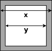
The problem has then three variables:

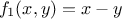which is called the thickness.
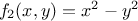which is called the section.
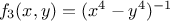which is called the distortion

and three natural constraints:

0 < < 1.
0 < < 1.
>

In the following sections the idea will be to study (if possible) the minimisation of the section of the bar and the distortion, keeping a minimum thickness of about 0.4. This threshold is chosen so that the bar can sustain its own weight. The examples will use an external code to compute the three previously-introduced variables once both the internal and external lengths are provided. The code is written in python as following:

#!/usr/bin/env python
"""
Simple file to mimick the barAllCost function to emulate it as a code
"""

x = .8
y = .3


def barre(out_l, in_l):
    """Compute the constraint and objectives for the hollow bar
    Arguments:
    out_l -- outter length of the hollow bar
    in_l -- inner length of the hollow bar
    """
    epais = out_l - in_l
    surf = out_l*out_l - in_l*in_l
    defor = 1 / (1.e-66 + out_l*out_l*out_l*out_l - in_l*in_l*in_l*in_l)
    return [epais, surf, defor]


def echo(out_l, in_l):
    """Print the results of the hollow bar computation
    Arguments:
    out_l -- outter length of the hollow bar
    in_l -- inner length of the hollow bar
    """
    print("#COLUMN_NAMES: c1|o1|o2")
    print("")
    evt = ""
    for i in barre(out_l, in_l):
        # print i,
        evt += "%.25g " % i
    print(evt)


echo(x, y)

In both examples, the same tip is used: the bar.py file is used to perform the computation (as the code is defined by python bar.py > output.dat) but it is also defined as the input file for the TCode. Thanks to this, the file is copied to every temporary working directory (so no need to change the $PYTHONPATH environment variable) and no extra file is needed to define the inputs. The output is directly stored as an ASCII file compatible with the usual Salome table format so that it can easily be read and convert as a TDataServer


Chapter IX. The Reoptimizer module		IX.3. Local solver