

Documentation
/ Manuel utilisateur en Python
: 
| Chapter XI. The Calibration module | ||
|---|---|---|
 |  | |
Table of Contents
This section presents different calibration methods that are provided to help achieve an accurate estimation of the parameters of a model with respect to data (either from experiment or from simulation). The methods implemented in Uranie are ranging from point estimation to more advanced Bayesian techniques and they mainly differ in the hypotheses they rely on.
They are all gathered in the libCalibration module. The namespace of this library is URANIE::Calibration. Each technique discussed later on is theoretically introduced in [metho] along with a general discussion on calibration and particularly on its statistical interpretation.
The reference data
will be compared with model predictions, where the model is a
mathematical function  . From now on and unless otherwise specified the
dimension of the output is set to 1 (
. From now on and unless otherwise specified the
dimension of the output is set to 1 ( ) which means
that the reference observations and the predictions of the model are scalars (the observations will then be written
) which means
that the reference observations and the predictions of the model are scalars (the observations will then be written
 and the predictions of the model
 ).
).
In addition to the problem-dependent
input vector, the model also depends on a parameter vector
 which is constant but unknown. The model is deterministic, meaning that is constant once both
  and
and  are fixed. In the rest of this documentation, a given set of parameter values
is called a configuration.
are fixed. In the rest of this documentation, a given set of parameter values
is called a configuration.
The rest of this section introduces the available distances and likelihoods used to compare observations with model predictions, in Section XI.1.1 while the methods are discussed in their own sections. The already predefined calibration methods proposed in the Uranie platform are listed below:
Minimisation techniques in Section XI.3
Analytical linear Bayesian estimation in Section XI.4
Approximate Bayesian Computation techniques (ABC) in Section XI.5
Markov chain Monte Carlo approach in Section XI.6
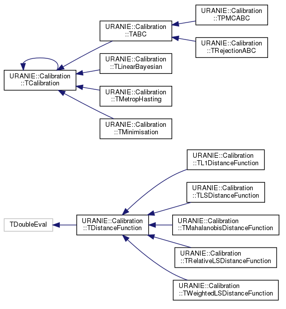
As for other modules, there is a specific class organisation that links the main classes in this module. The class hierarchy
is shown in Figure XI.1 and is discussed a bit here to explain the two main classes from
which all other classes are derived and the corresponding shared functions used throughout the methods. One can see this organisation
with the two sets of classes: those inheriting from the TCalibration class and those inheriting from
TDistanceFunction class. The former are the different methods that have been developed to calibrate a
model with respect to the observations and each method will be discussed in the upcoming sections. Whatever the method under
consideration, it always includes a distance or a likelihood function object, which belongs to the latter category and its main
job is to quantify how close the model predictions are to the observations. These objects are discussed in the rest of this
introduction, see for instance Section XI.1.1.
Although CIRCE is not strictly a calibration method, it has been included in this section because it relies on approaches
presented here. Indeed, the idea behind this method is to quantify the uncertainty of a given quantity by multiplying it by a
Gaussian random variable whose standard deviation must be calibrated. A final section therefore introduces this method.
CIRCE method in Section XI.7
The next section focuses on the distances and likelihoods already implemented in Uranie, which can be used directly within the calibration methods.
There are many ways to quantify the agreement between the reference observations and the model predictions, given a
parameter vector . Depending on the framework adopted (deterministic or Bayesian), different tools are required. In a
deterministic setting, a distance is used to measure how far the prediction is from the observation. In contrast,
within the Bayesian framework, the analogous concept is the likelihood, a function that evaluates the probability of
observing the data given a parameter vector.
Since the number of variables  used to perform the calibration can be greater than one, it might be useful to introduce the coefficients
 to weight the contribution of each variable relative to the others. The following lists the distance functions available in Uranie:
L1 distance function (sometimes called Manhattan distance):
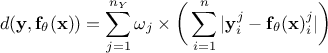 ;
;
Least squares distance function:
;
Relative least squares distance function:
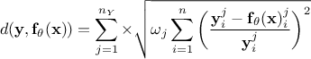 ;
;
Weighted least squares distance function:
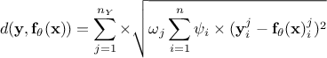 , where the coefficients
 are associated with the j-th variable and are used to weight each observation with respect to the others;
Mahalanobis distance function:
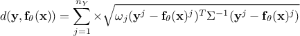 where
where  is the covariance matrix of the observations.
Regarding the likelihood functions already implemented, only the Gaussian log-likelihood for independent parameters is available, as it is the most commonly used. Its expression follows:
Gaussian log-likelihood for independent parameters:
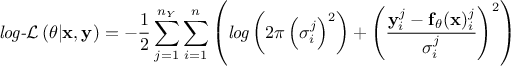 where the
coefficients
where the
coefficients  are the standard deviations of each observation associated to the j-th variable.
If needed, it is still possible to define a custom likelihood (or distance).
For more details on the implementation of the distances and likelihoods, or on how to implement your own, see Section XI.2.2.
| | | |
| X.2. Efficient Global Optimization |  | XI.2. Calibration classes, distance and likelihood functions, observations and model |