Documentation / User's manual in Python :

XI.2. Calibration classes, distance and likelihood functions, observations and model

XI.2. Calibration classes, distance and likelihood functions, observations and model
	Chapter XI. The Calibration module

XI.2. Calibration classes, distance and likelihood functions, observations and model

This section introduces the common elements of all analyses in the Calibration module. Indeed the methods discussed hereafter will be using the same architecture and will require a common set of items, listed below:

a model has to be set up as this is what one wants to calibrate. It can come either as a Relauncher::TRun instance, as a Launcher::TCode or a Launcher function. This part is introduced in Section XI.2.1 (for the general concept and the difference with the usual organisation of model definition) and discussed later on (mainly in relation to the constructor of TCalibration-derived objects) in Section XI.2.3 and in the dedicated section in each method;
a reference observations have to be defined once and for all so that the model can be run for each newly defined set of parameter values (every new configuration). This part is discussed first in Section XI.2.1 and the way to provide them is also partly discussed in Section XI.2.2;
a distance or likelihood function has to be created, usually within the calibration instance, to quantify how well the model under study reproduces the reference observations. This part is discussed in Section XI.2.2.
a main object has to be created, a calibration method instance, that inherits from the TCalibration class. This is discussed in Section XI.2.3.

XI.2.1. General introduction to data and model definition

All calibration problems will have at least two TDataServer objects:

The reference one, usually called tdsRef, contains the observations (both input and output attributes) on which the calibration is to be performed. It is generally read from a simple input file as done below:
```
tdsRef = DataServer.TDataServer("reference", "my reference")
tdsRef.fileDataRead("myInputData.dat")
              
```
the parameter one, usually called tdsPar, contains only attributes and must be empty of data. Its purpose is to define the parameters that should be tested in the calibration process and, depending on the method chosen, will only contain TAttribute members (for minimisation, see Section XI.3) or only TStochasticAttribute inheriting objects for all other methods. The latter case gathers the method doing the analytical computation when the chosen priors are allowed (see Section XI.4) along with all those that require generating one or more design-of-experiments (see Section XI.5 but also Section XI.6).

This step, which should represent the first lines of the calibration procedure, goes along with the model definition. This one is tricky with respect to all the examples provided in Section XIV.5 and in Section XIV.9 as the inputs of the model are coming from two different TDataServers, they can be split into two categories:

the reference ones will only have values from the reference input file myInputData.dat, which contains observations. For each configuration, the model is evaluated times: the configuration remains fixed, while the reference values are varied across those observations;
the parameter ones, on the other hand, change only when moving to a new configuration and remain constant across all reference evaluations.

Depending on the way the model is coded (and more likely on the parameters the user would like to calibrate) these attributes might not be separated in terms of order, meaning that the list of inputs of a model might look a bit like this:


# Example of input list for a fictive model (whatever the launching solution is chosen)
# ref_var1, ref_var2, ref_var3, ref_var4 are coming from the tdsRef dataserver
# par1, par2 are coming from the tdsPar dataserver 
sinputList = "ref_var1:par_1:ref_var2:ref_var3:ref_var4:par_2"

Warning

As a result, there is no implicit declaration allowed in the calibration classes constructor and particular attention must be paid when defining the model: the user must provide the list of inputs (for Launcher-type model) or fill the input and output list into the TEval-inheriting object in the correct order (for Relauncher-type model). This is further discussed in Section XI.2.3.

Finally, all models considered for calibration should have exactly as many outputs (whatever their names are) as the number of outputs to be compared with (the output attributes in the tdsRef TDataServer object). These outputs are those that will be used to compute the chosen agreement (meaning the result of the distance or likelihood function which is the only quantifiable measurement we have between the reference and the predictions for a given configuration). At the end of a calibration process, the user can find three different kinds of information (more can be added if needed, see Section XI.2.3.4):

the resulting calibrated value of the parameters (or values depending on the chosen method, as some of them are providing several samples of calibrated configurations) is being stored in the parameter TDataServer object: as this object was provided empty and should contain only an attribute per parameter to be calibrated, it seems be the best place to store results. This is obviously the expected target but it should not be considered conclusive without having a look at the two other ones;
the agreement between the reference data and the model predictions, which are stored in the parameter TDataServer object tdsPar for every calibrated configuration;
the residuals: the difference between the model predictions and the reference data for the observations, using the a priori and a posteriori configurations. These are stored in a dedicated TDataServer object, called the EvaluationTDS (referred to as tdsEval) and it is mainly called through the drawResiduals method (discussed in Section XI.2.3.7). If one wants to access it, it is possible to get a hand on it by calling the getEvaluationTDS() method. The residuals are important to check that the behaviour of the newly performed calibration does not show unexpected and unexplained tendencies with respect to any variables in the defined uncertainty setup, see the dedicated discussion on this in [metho]

XI.2.2. Defining data, distance and likelihood functions

The different distance and likelihood functions already embedded in Uranie can be found in Section XI.1.1 and are further discussed from a theoretical point of view in[metho]. From the user point of view, on the other hand, every distance or likelihood function inherits from the class TDistanceLikelihoodFunction, as can be seen in Figure XI.1, which is purely virtual (meaning that no object can be instantiated as TDistanceLikelihoodFunction) and serves several main purposes:

it loads the reference data once and stores them internally as a vector of vectors (or as a vector of TMatrixD depending on the chosen formalism used to compute the distance or likelihood);
once done, the following loop is executed as long as new configurations need to be tested (a configuration being defined as a new set of values for vector ):
1. it runs the chosen model regardless of the nature of the object (TRun, TCode, etc.) on the full reference dataset to get the new predictions;
2. it loads the new model predictions for the configuration under study into a vector of vectors (or as a vector of TMatrixD depending on the chosen formalism);
3. it computes the distance or likelihood using both vectors as statd by the equations in Section XI.1.1. This computation is done within the localeval method (which is the only method that should be redefined if a user wants to create its own distance or likelihood function, see dedicated discussion in Section XI.2.2.2).

From a technical point of view, the TDistanceLikelihoodFunction inherits from the TDoubleEval class which is a part of the Relauncher module. This inheritance is not very important as its main appeal is to considerably simplify the implementation of the minimisation methods with the Reoptimizer module, allowing the straightforward use of all TNlopt algorithms as well as Vizir solutions (see Section XI.3).

Regardless of the calibration method considered, a distance or likelihood function must be used to compare data and model predictions. This is even true for the TLinearBayesian class, which directly computes the analytical posterior distribution, as the residuals are computed both a priori and a posteriori to assess the improvement of the prediction and their consistency within the uncertainty model (see discussion in [metho]). In most cases the object will be constructed with a recommended way (discussed in Section XI.2.2.1). Another possibility is also discussed in Section XI.2.2.2

Whatever the situation, once a calibration instance is created (for the sake of generality, we will use an instance named cal, of the mock class TCalClass as if it inherited from the TCalibration class), the first method to be called is the setDistance or setLikelihood, depending on the framework used (see the corresponding section), as this is the method which defines both the type of distance or likelihood function and the observation dataset.

XI.2.2.1. Recommended distance and likelihood functions, construction method

There are several ways to define a distance or a likelihood function. The recommended approach is to use the setDistance and setLikelihood methods, which are directly available in each calibration class such as TLinearBayesian or TMinimisation. Alternatively, one can call setDistanceAndLikelihood method from the TCalibration class (which is actually invoked by the two previous methods), and is inherited by all calibration classes. However, we recommend using the first two approaches, in order to prevent mistakenly assigning distances to likelihood-based methods, or likelihood functions to distance-based methods. The prototypes discussed here are as follows:


setDistanceAndLikelihood(funcName, tdsRef, input, reference, weight="")
setDistance(funcName, tdsRef, input, reference, weight="")
setLikelihood(funcName, tdsRef, input, reference, weight="")

It takes up to five arguments, one of which is optional:

funcname: the name of the distance or likelihood function, corresponding to one of the already implemented one, as discussed in Section XI.1.1. The possible choices are
- "L1" for TL1DistanceFunction;
- "LS" for TLSDistanceFunction;
- "RelativeLS" for TRelativeLSDistanceFunction;
- "WeightedLS" for TWeightedLSDistanceFunction;
- "Mahalanobis" for TMahalanobisDistanceFunction;
- "log-gauss" for TGaussLogLikelihoodFunction.
tdsRef: the TDataServer in which the observations are stored;
input: the input variables stored in the TDataServer tdsRef, which must be defined as inputs in the code before creating the calibration object. This argument has the usual attribute list format "x:y:z";
reference: the reference variables stored in the TDataServer tdsRef, against which the output of the code or function will be compared. This argument has the usual attribute list format "out1:out2:out3";
weight (optional): this argument is optional and can be used to define the name of the (single) variable stored in the TDataServer tdsRef which, in the case of a TWeightedLSDistanceFunction, is used to fill the , i.e. the coefficients that weight each observation relative to the others and, in the case of a TGaussLogLikelihoodFunction, is used to fill the , i.e. the standard deviations of each observation associated to the j-th variable (see Section XI.1.1).
Warning
The number of variables in the weight list should match the number of outputs of your code used to calibrate the parameters. If one output is not weighted, a "one" attribute should be added to handle that output, when the other requires an uncertainty model.

Once this method is called, the distance or likelihood function is created and is stored within the calibration object. It may be necessary to access it for certain options, but this is further discussed in Section XI.2.2.3.

The following line summarises this construction in a case where an instance cal of the fake class TCalClass (as if this class was inheriting from the TCalibration class) is created.


# Define the dataservers
tdsRef = DataServer.TDataServer("reference", "myReferenceData")
# Load the data, both inputs (ref_var1 and ref_var2) and a single output (ref_out1).
tdsRef.fileDataRead("myInputData.dat")
...
tdsPar = DataServer.TDataServer("parameters", "myParameters")
tdsPar.addAttribute(DataServer.TNormalDistribution("par1", 0, 1))
# the parameter to calibrate
...
# Define the model
...
# Create the instance of TCalClass
cal = Calibration.TCalClass()  # Constructor is discussed later on
# Define the least squares distance
cal.setDistance("LS", tdsRef, "ref_var1:ref_var2", "ref_out1")

In this fake example, the distance function is the least squares one, and it will use the values of both inputs "ref_var1" and "ref_var2" and output "ref_out1" stored in tdsRef to calibrate the parameter "par1". No observation weight is needed in this case, as least squares method does not require it and as there is only a single output, no variable weight needs to be defined either.

XI.2.2.2. Creating its own distance or likelihood function

It is possible to create a custom distance or likelihood function if one wants to use a function not already implemented in Uranie.

XI.2.2.3. Available options for every distance and likelihood function

All distance and likelihood function classes inherit from TDistanceLikelihoodFunction, and the only difference among them lies in the implementation of the localeval function. As a result, a large portion of the code is shared across all the distance and likelihood function objects, including the parts handling their configuration and options.

This subsection gathers all the shared options, which can be configured either through the optional "Option" parameter in several methods and constructors, or by accessing the distance or likelihood function object directly once it has been created. To do so, the user can call the getDistanceLikelihoodFunction method, which returns the distance or likelihood function instance stored within the calibration object. The following lines provide an example using an instance cal of the mock class TCalClass (as if it were inheriting from the TCalibration class).


# import rootlogon to get Calibration namesppace
from rootlogon import DataServer, Calibration
# ....            
# Creating the calibration instance from a TDataServer and a Relauncher::TRun           
cal = Calibration.TCalClass(tdsPar, runner, 1, "")
# Creating the distance function (a least square one)
cal.setDistance("LS", tdsRef, "logRe:logPr", "logNu")
# Retrieving the instance to be able to change options
dFunc = cal.getDistanceLikelihoodFunction();()

XI.2.2.3.1. Defining the variable weights

When multiple variables are used to compare predictions with observations, it may be desirable to weight their respective contributions to the distance. This is precisely the purpose of the variable described in Section XI.1.1. This option is not relevant for the Gaussian log-likelihood, since the "contribution" of the variables are already weighted by the standard deviation (through the uncertainty on the data). For all distances, two different methods are available to define some variable weights, both called setVarWeights. The only difference lies in their prototype :


# Prototype 1 with array defined as
# wei = np.array([0.5, 0.4])
setVarWeights(len(wei), wei)
# Prototype 2 with vectors defined as
# wei = ROOT.std.vector['double']([0.5, 0.4])
setVarWeights(wei)

The idea behind these two prototypes is to have a way to control the number of elements in the array of doubles, either by asking the user to provide it (in prototype 1) or as a by-product of the vector structure. From there, if the size of the array matches the number of output variables the weights are initialised; otherwise, the program will crash.

XI.2.2.3.2. Dumping all the estimates

Whatever the construction and evaluation type (either based on Launcher or Relauncher), you might want to keep track of all evaluations across all the reference observations and not only the global distance or likelihood. This is possible by calling the dumpAllDataservers method of TDistanceLikelihoodFunction:


dumpAllDataservers()

This method takes no arguments and sets a boolean to true (by default it is set to false) which implies that every configuration will be dumped as an ASCII file that will be named according to the following convention: Calibration_testnumber_XX.dat where XX is the configuration number for the under-study analysis.

Warning

This option might dump a very large number of files which can fill your local disk (for instance, if you are testing functions where the limit on the number of configurations is not strictly enforced). When used with a runner architecture (Relauncher-type evaluator), the parameters are not kept by default in the dataserver (they are defined as ConstantAttribute). To get the required behaviour (i.e., including the parameter values in the ASCII file), the user should also call the keepParametersValue method of TDistanceLikelihoodFunction:


keepParametersValue()

This function, which takes no argument, simply sets to true the final argument of all TLauncher2 calls to addConstantAttribute.

XI.2.2.3.3. Defining the observations covariance matrix

In the case where the observations are correlated with a known covariance structure, this covariance can be specified as a TMatrixD using the following method:


setObservationCovarianceMatrix(mat)

This method, and the ability to define a covariance structure between observations, is only relevant when the distance function is an instance of the TMahalanobisDistanceFunction.

XI.2.2.3.4. Specifying a Launcher object or options

This method is very specific as it can be used for all calibration classes, but only if the model introduced is a Launcher::TCode. This option appears here, because the distance or likelihood function is the place where the model is used to estimate the new predictions for a newly set parameter vector (see Section XI.2.2). This option allows not to use the usual TLauncher object in order to use one of the other instances. This is done in a single function:


changeLauncher(tlcName)

The only argument of this method is a TString object which is used to select one of the two other instances in the Launcher module for the TCode: either the TLauncherByStep or the TLauncherByStepRemote. When used, the setDrawProgressBar method is also called to set this variable to false.

The main point of this is to switch from a usual TLauncher object to another one chosen by the user. Among the possible solutions one can set

TLauncherByStep: if the user wants to break down the launching process, decomposing it into preTreatment, run, and postTreatment.
TLauncherByStepRemote: if the user wants to use the code on a cluster on which Uranie is not installed. This is not recommended for any cluster setup, such as the CEA clusters. This is based on the libssh library, see Section IV.4.5 for more details.

Finally, the default option for the run method of any TLauncher-inheriting instance is noIntermediateSteps, which prevents the safe writing of the results into a file every five estimates. Two methods can be applied on TDistanceLikelihoodFunction objects to change these options:


# Adding more options to the code launcher run method
addCodeLauncherOpt(opt)
# Change the code launcher run method options
changeCodeLauncherOpt(opt)

The first one keeps the default options and adds more on top, for instance options that would allow to distribute the computation with the fork process (as a reminder, this option is "localhost=X" where X stands for the number of threads to be used). On the other hand, the second method allows restarting from scratch in order to define the options as chosen by the user.

XI.2.2.3.5. Dumping the distance details

In the case where one does not understand or trust the way the distance or likelihood is computed, it is possible to dump the details of their computation (warning: this is very verbose). This can be done by calling the dumpDetails, whose prototype is straightforward:


dumpDetails()

XI.2.3. Common methods of the calibration classes

All calibration classes that derive from TCalibration share many common methods, and their organisation has been streamlined as much as possible. This section describes the shared code to avoid repetition in the later sections, which cover each specific calibration method (from Section XI.3 to Section XI.6).

The subsections from Section XI.2.3.1 to Section XI.2.3.3 discuss the different constructors, explaining the various ways the model can be provided and their implications while Section XI.2.3.4 provides a glimpse of the shared possible options that can be defined and their purpose. Finally, Section XI.2.3.6 and Section XI.2.3.7 introduce the drawing methods in principle (though illustrations are postponed to dedicated sections of this documentation).

Warning

As with some earlier discussions, the following methods are common to all classes inheriting from TCalibration. For illustration, the examples will use an instance cal of the fictitious class TCalClass (as if it inherited from TCalibration class). A more realistic syntax can be found in the dedicated sections (from Section XI.3 to Section XI.6).

Calibration classes can generally be constructed in four different ways, depending on how the model has been specified. To estimate how close the new set of parameter values (the configuration) produces output that are close to the reference, one needs to be able to run the model on the input variables of the reference dataset. The input variables of the reference dataset are not the only input variables of the model used within the calibration method, as the parameters themselves have to be specified as inputs (as they also obviously affect the predictions). This section illustrates, using the fictitious class TCalClass how calibration objects can be constructed.

XI.2.3.1. Construction with a `TRun`

This constructor uses the Relauncher architecture. This approach provides a simple way to change the evaluator (e.g., switching from a C++ function to a Python function or another code). It also allows the use of either a sequential approach (for single-thread execution) or a threaded approach (to distribute estimates locally). This approach is partly discussed in Chapter VIII.

In this case, the constructor has the following form:


# Constructor with a runner
TCalClass(tds, runner, ns=1, option="")

It takes up to four arguments, two of which are optional:

tds: a TDataServer object containing one attribute for each parameter to be calibrated. This is the TDataServer object called tdsPar, defined in Section XI.2.1.
runner: a TRun-inheriting instance that contains all the model information and whose type determines how the estimates are distributed: it can either be a TSequentialRun instance or TThreadedRun for distributed computations.
ns (optional): the number of samples to be produced. This parameter is only relevant for methods that return multiple configurations (either multiple solutions to the minimisation problem or samples from the posterior distribution). It is not used in local minimisation with single-point initialisation, nor in linear Bayesian analysis (see Section XI.4). The default value is 1.
option (optional): the options that can be applied to the method. Options common to all calibration classes (those defined in the TCalibration class) are discussed in Section XI.2.3.4.

A crucial step in this constructor is the creation of the instance that inherits from TRun. As mentioned earlier, its type determines how the estimates are distributed. To construct such an object, one needs to provide an evaluator (the available evaluators are described in detail in Section VIII.3).

Using the formalism introduced in Section XI.2.2.1, a model instance based on the code Foo, initialised with TCIntEval, can be created as shown below. This example assumes the model takes three inputs ("ref_var1", "par1", "ref_var2") and it produces a single output, which is compared with the reference output "ref_out1" via the distance or likelihood function (see Section XI.2.2.1).


# Define the dataservers
tdsRef = DataServer.TDataServer("reference", "myReferenceData")
# Load the data, both inputs (ref_var1 and ref_var2) and a single output (ref_out1).
tdsRef.fileDataRead("myInputData.dat")
...
TDataServer *tdsPar = new TDataServer("parameters", "myParameters")
tdsPar.addAttribute(DataServer.TNormalDistribution("par1", 0, 1))  # parameter to calibrate
...
# Define the model if a function Foo is loaded through ROOT.gROOT.LoadMacro(...)
# for which x[0]=ref_var1, x[1]=par1 and x[2]=ref_var2 and y[0] is the model prediction
model = Relauncher.TCIntEval(Foo)
# Add inputs in the correct order
model.addInput(tdsRef.getAttribute("ref_var1"))
model.addInput(tdsPar.getAttribute("par1"))
model.addInput(tdsRef.getAttribute("ref_var2"))
# Define the output attribute
out = DataServer.TAttribute("out")
model.addOutput(out)
# Define a sequential runner to be used
runner = Relauncher.TSequentialRun(model)    
...
# Create the instance of TCalClass
ns = 1
cal = Calibration.TCalClass(tdsPar, runner, ns, "")

XI.2.3.2. Construction with a `TCode`

This constructor uses the Launcher architecture. Unlike the Relauncher approach, it is specifically designed for code-based models.

In this case, the constructor has the following form:


# Constructor with a TCode
TCalClass(tds, code, ns=1, option="")

It takes up to four arguments, two of which are optional:

tds: a TDataServer object containing one attribute for each parameter to be calibrated. This is the TDataServer object called tdsPar, defined in Section XI.2.1.
code: a TCode instance containing the output file (or files) listing the output attributes while all input attributes are associated with input files using the standard methods (setFileKey, setFileFlag, etc.).
ns (optional): the number of samples to be produced. This parameter is only relevant for methods that return multiple configurations (either multiple solutions to the minimisation problem or samples from the posterior distribution). It is not used in local minimisation with single-point initialisation, nor in linear Bayesian analysis (see Section XI.4). The default value is 1.
option (optional): the option that can be applied to the method. Options common to all calibration classes (those defined in the TCalibration class) are discussed in Section XI.2.3.4.

Unlike the runner-based constructor, this construction does not define how the computation is performed. By default, the run method is called for each configuration with the following options:

noIntermediateSteps: prevents results from being saved every five estimates.
quiet: suppresses verbose output from the launcher.

Two methods can be applied on TDistanceLikelihoodFunction objects to change these options: addCodeLauncherOpt and changeCodeLauncherOpt (see Section XI.2.2.3.4).


# Adding more options to the code launcher
addCodeLauncherOpt(opt)
# Change the code launcher option 
changeCodeLauncherOpt(opt)

The first method retains the default configuration and appends additional options, for example an option that enables distributed computation using the fork process (recall that this option is "localhost=X", where X denotes the number of threads to use). In contrast, the second method resets the configuration entirely, allowing the user to define a new set of options from scratch.

Using the formalism introduced in Section XI.2.2.1, a model instance based on the code Foo, initialised with TCode, can be created as shown below. This example assumes the model takes three inputs ("ref_var1", "par1", "ref_var2") and it produces a single output, which is compared with the reference output "ref_out1" via the distance or likelihood function (see Section XI.2.2.1).


# Define the dataservers
tdsRef = DataServer.TDataServer("reference", "myReferenceData")
# Load the data, both inputs (ref_var1 and ref_var2) and a single output (ref_out1).
tdsRef.fileDataRead("myInputData.dat")
...
tdsPar = DataServer.TDataServer("parameters", "myParameters")
tdsPar.addAttribute(DataServer.TNormalDistribution("par1", 0, 1))  # parameter to calibrate
...
sIn = TString("code_foo_input.in")
# Set the reference input file and the key for each input attributes
tdsRef.getAttribute("ref_var1").setFileKey(sIn, "var1")
tdsRef.getAttribute("ref_var2").setFileKey(sIn, "var2")
tdsPar.getAttribute("par1").setFileKey(sIn, "par1")
# The output file of the code
fout = Launcher.TOutputFileRow("_output_code_foo_.dat")
# The attribute in the output file
fout.addAttribute(DataServer.TAttribute("out"))
# Creation of the code
mycode = Launcher.TCode(tdsRef, "foo -s -k")
mycode.addOutputFile( fout )
...
# Create the instance of TCalClass
int ns=1
cal = Calibration.TCalClass(tdsPar, mycode, ns, "")

XI.2.3.3. Construction for a function with the Launcher architecture

This constructor uses the Launcher architecture and is designed for C++ functions with the standard prototype.

In this case, the constructors have the following forms:


# Constructor with a function pointer using Launcher
TCalClass(tds, fcn, varexpinput, varexpoutput, ns=1, option="")
# Constructor with a function name using Launcher            
TCalClass(tds, fcn, varexpinput, varexpoutput, ns=1, option="")

It takes up to six arguments, two of which are optional:

tds: a TDataServer object containing one attribute for each parameter to be calibrated. This is the tdsPar, defined in Section XI.2.1.
fcn: the second argument is either the name of the function or a pointer to this function. The user must know the exact order of the input and output variables of this function.
varexinput: a colon-separated list of input variables, in the correct order, mixing reference attributes and parameter attributes.
varexpoutput: a colon-separated list of output variables.
ns (optional): the number of samples to be produced. This parameter is only relevant for methods that return multiple configurations (either multiple solutions to the minimisation problem or samples from the posterior distribution). It is not used for local minimisation with single-point initialisation, nor for linear Bayesian analysis (see Section XI.4). The default value is 1.
option (optional): the option that can be applied to the method. Options common to all calibration classes (those defined in the TCalibration class) are discussed in Section XI.2.3.4.

This is the simplest constructor: all information is provided in a single line, no extra options need to be defined, and no files must be created. Using the formalism introduced in Section XI.2.2.1, the calibration object can be constructed using a function-pointer prototype of the code Foo as shown below. This example assumes the model takes three inputs ("ref_var1", "par1", "ref_var2") and it produces a single output, which is compared with the reference output "ref_out1" via the distance or likelihood function (see Section XI.2.2.1).


# Define the dataservers
tdsRef = DataServer.TDataServer("reference","myReferenceData")
# Load the data, both inputs (ref_var1 and ref_var2) and a single output (ref_out1).
tdsRef.fileDataRead("myInputData.dat")
...
tdsPar = DataServer.TDataServer("parameters","myParameters")
tdsPar.addAttribute(DataServer.TNormalDistribution("par1", 0, 1))  # parameter to calibrate
...
# Create the instance of TCalClass
ns = 1
cal = Calibration.TCalClass(tdsPar, Foo, "ref_var1:par1:ref_var2", "out", ns, "")

XI.2.3.4. Running the estimate

Once the calibration object is constructed and its distance or likelihood function created, the next step is to perform the calibration, that is to estimate the best value(s) or distribution of the parameters given the data. This is done by calling the method


estimateParameters(option="")

This method is generic and primarily calls an internal method, implemented in each class inheriting from TCalibration, where the actual estimate is performed.

There are different options that can be applied to the estimateParameters method, among which:

"saveAllEval": keeps all individual estimates in the internal dataserver, which can later be used to produce residuals plots (see Section XI.2.3.7). This may become impractical, as the number of stored estimates can be extremely large;
"noAgreement": this options removes the agreement attribute at the end of the estimate, if that information is deemed unnecessary.

Additional options, triggered via methods of the TDistanceLikelihoodFunction-inheriting instances, may also be useful for understanding and validating the calibration. For details, see Section XI.2.2.3.

Several methods are available to represent the results. Their basic structure is defined in the TCalibration class, though some may not apply to specific methods. This section introduces the general framework while method-specific details are discussed in their respective sections.

XI.2.3.5. Estimate custom residuals

Once the estimate has been performed, both a priori and a posteriori residuals can be computed. Since a priori and a posteriori estimates depend on the chosen algorithm, their formulas are not detailed here. It is also possible to re-evaluate residuals for any custom set of parameter values provided by the user. This can be done through


estimateCustomResiduals(resName, theta_nb, theta_val)

It takes three arguments, which are:

resName: a tag identifying the stored set of residuals;
theta_nb: the number of parameter values in the array (must match _nPar);
theta_val: an array containing the parameter values.

For convenience, this method can be called with a numpy array, as shown below


import numpy as np
mypar = np.array([0., 2., 3.])
mycal.estimateCustomResiduals("set1", len(mpar), mypar)

This feature allows re-estimating the residuals based on the available sample after the a posteriori values distributions have been calibrated. A common use case is Markov chain Monte Carlo methods, where it may be necessary to discard the burn-in phase before evaluating residuals. Once created, the custom set can be used in the drawResiduals function, as discussed in Section XI.2.3.7.

XI.2.3.6. Drawing the parameters

This method is used to visualize parameter values and posterior samples. The prototype is:


drawParameters(sTitre, variable = "*", option = "")

It takes up to three arguments, two of which are optional:

sTitre

the title of the plot (an empty string is allowed);

variable (optional)

a list of parameter names to be drawn, separated by colons ":". The default "*" draws all parameters;

option (optional)

a list of options, separated by commas "," to adjust the plotting behavior:

"nonewcanvas": draw on the current canvas (instead of creating a new one);
"vertical": if multiple parameters are plotted, display them stacked vertically (one per row). By default, plots are arranged horizontally, side by side.

Warning

If the TMCMC calibration object is used, the drawParameters method accounts for the potential burn-in and lag values by discarding the initial samples of the Markov chain and thinning it according to the specified values, in order to properly represent the behavior of the posterior distribution (see Section XI.6).

XI.2.3.7. Drawing the residuals

This method is used to visualize the residuals of the output variables, i.e. the discrepancies between the model predictions and the reference outputs. Two types of residuals are typically considered:

A priori residuals - based on the initial parameter values or the prior distribution;
A posteriori residuals - obtained after the calibration procedure.

The prototype is:


drawResidues(sTitre, variable = "*", select="1>0", option = "")

It takes up to four arguments, three of which are optional:

sTitre

the title of the plot (an empty string is allowed);

variable (optional)

a list of parameter names for which one wants to draw the residuals, separated by colons ":". The default "*" draws all parameters;

select (optional)

a selection expression that filters out configurations. For example, it can be used to exclude the burn-in period or to apply lag procedures in the MCMC algorithms (see Section XI.6);

option (optional)

a list of options, separated by commas "," to adjust the plotting behavior:

"nonewcanvas": draw on the current canvas (instead of creating a new one);
"vertical": if multiple parameters are plotted, display them stacked vertically (one per row). By default, plots are arranged horizontally, side by side.
"apriori/aposteriori": draw only the a priori residuals or only the a posteriori residuals. If neither option is specified, both are displayed;
"custom=XXX": also draw custom residuals computed with estimateCustomResiduals.

For example, using the custom set "set1" defined earlier (see Section XI.2.3.5), one can compare a priori, a posteriori, and custom residuals:


mycal.drawResiduals("Residuals title", "*", "", "nonewcanvas,apriori,aposteriori,custom=set1")

Summary: TCalibration and TDistanceLikelihoodFunction

In summary, a calibration analysis should always follow these key steps:

Define both the parameter (tdsPar) and reference (tdsRef) objects, as explained in Section XI.2.1.
Define the model architecture (either Relauncher or Launcher-based) and the evaluator kind (code, C++-function, python-function...). Particular attention is needed when specifying the input and output attributes (the former should be an admixture of attributes from tdsPar and tdsRef, as explained in Section XI.2.1.
Define the TCalibration-inheriting object (meaning the underlying method chosen for this analysis) and construct it (see from Section XI.2.3.1 to Section XI.2.3.3).
Define the TDistanceLikelihoodFunction-inheriting object by calling setDistance or setLikelihood (depending on the TCalibration object), see the recommended distance and likelihood functions in Section XI.2.2.1.
Set the method-dependent parameters (discussed in dedicated part, from Section XI.3 to Section XI.6).
Call the estimateParameters method with selected options (see Section XI.2.3.4).
Perform the post-processing using method-dependent functions discussed in the dedicated sections, from Section XI.3 to Section XI.6) and drawing methods (see also both Section XI.2.3.6 and Section XI.2.3.7).

XI.2.4. Use-case for this chapter

To illustrate the methods discussed in the following sections, in more detail than the previously introduced dummy examples, a general use-case will be used. This use-case relies on the flowrate model introduced (along with a descriptive sketch) in Chapter IV and whose equation is recalled below:

Equation XI.1.

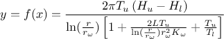
where the eight parameters are:

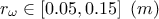: radius of borehole;
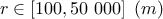: radius of influence;
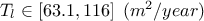
: Transmitivity of the superior layer of water;
: Transmitivity of the inferior layer of water;
: Potentiometric "head" of the superior layer of water;
: Potentiometric "head" of the inferior layer of water;
: length of borehole;
: hydraulic conductivity of borehole.

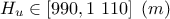
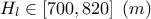
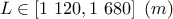
This example has been treated by several authors in the dedicated literature, for instance in [worley1987deterministic]. For our purposes, the idea behind the upcoming examples (in this chapter, along with those in the use-case section, see Section XIV.12) is to consider that one has an observation sample. For this function, we consider that from all the inputs, only two have been varied ( and ) and only one is actually unknown: . The rest of the variables are set to fixed values: , , , , . This can be written as the following function (using the usual C++ prototype)


void flowrateModel(double *x, double *y) 
{
  double rw = x[1], r = 25050;
  double tu = 89335, tl = 89.55;
  double hu = 1050, hl = x[0];
  double l = x[2], kw = 10950;

  double num = 2.0 * TMath::Pi() * tu * (hu - hl);
  double lnronrw = TMath::Log(r / rw);
  double den = lnronrw * (1.0 + (2.0 * l * tu) / (lnronrw * rw * rw * kw) + tu / tl);

  y[0] = num / den;
}

As discussed previously, the function assumes that the user is aware of the input order. In this case, the parameter to be calibrated () comes first while the varying inputs ( and ) come later. The first lines of all examples should look like this


# Name of the input reference file
ExpData = "Ex2DoE_n100_sd1.75.dat"

# Define the reference
tdsRef = DataServer.TDataServer("tdsRef", "doe_exp_Re_Pr")
tdsRef.fileDataRead(ExpData)

# Define the parameters
tdsPar = DataServer.TDataServer("tdsPar", "pouet")
tdsPar.addAttribute(DataServer.TAttribute("hl", 700.0, 760.0))  # if stochastic laws are needed
# use tdsPar.addAttribute(DataServer.TUniformDistribution("hl", 700.0, 760.0))

# Create the output attribute
out = DataServer.TAttribute("out")


Chapter XI. The Calibration module		XI.3. Minimisation techniques

Documentation / User's manual in Python :

XI.2. Calibration classes, distance and likelihood functions, observations and model

XI.2.1. General introduction to data and model definition

Warning

XI.2.2. Defining data, distance and likelihood functions

XI.2.2.1. Recommended distance and likelihood functions, construction method

Warning

XI.2.2.2. Creating its own distance or likelihood function

XI.2.2.3. Available options for every distance and likelihood function

XI.2.2.3.1. Defining the variable weights

XI.2.2.3.2. Dumping all the estimates

Warning

XI.2.2.3.3. Defining the observations covariance matrix

XI.2.2.3.4. Specifying a Launcher object or options

XI.2.2.3.5. Dumping the distance details

XI.2.3. Common methods of the calibration classes

Warning

XI.2.3.1. Construction with a TRun

XI.2.3.2. Construction with a TCode

XI.2.3.3. Construction for a function with the Launcher architecture

XI.2.3.4. Running the estimate

XI.2.3.5. Estimate custom residuals

XI.2.3.6. Drawing the parameters

Warning

XI.2.3.7. Drawing the residuals

XI.2.4. Use-case for this chapter

XI.2.3.1. Construction with a `TRun`

XI.2.3.2. Construction with a `TCode`