

Documentation
/ Manuel utilisateur en Python
: 
| XI.5. Approximate Bayesian Computation techniques (ABC) | ||
|---|---|---|
 | Chapter XI. The Calibration module |  |
This section covers methods grouped under the acronym ABC, which stands for Approximate Bayesian Computation. The core idea is to perform Bayesian inference without explicitly evaluating the model likelihood function. For this reason, these methods are also refered to as likelihood-free algorithms [wilkinson2013approximate].
As a reminder, the principle of the Bayesian approach is summarized in the equation
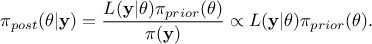 , where
  is the conditional probability of the observations given the parameter values
  ,
,  is the a
priori probability density of (the prior), and
is the a
priori probability density of (the prior), and  is the marginal likelihood of the observations, which is constant.
For more details, see
[metho].
is the marginal likelihood of the observations, which is constant.
For more details, see
[metho].
From a technical perspective, the methods in this section inherit from the TABC class (which
itself inherits from TCalibration, in order to benefit from all standard features).
Currently, the only implemented ABC method is the Rejection algorithm, presented in [metho], whose implementation is
provided through the TRejectionABC class described below.
The usage of the TRejectionABC class can be summarised in a few key steps:
Prepare the data and the model:
The parameters to be calibrated must be instances of classes inheriting from
TStochasticAttribute;Select the assessor type and construct the
TRejectionABCobject with the appropriate distance function (see Section XI.5.1).
Set the algorithm properties:
Define optional behaviours;
Specify the uncertainty hypotheses via the dedicated methods (see Section XI.5.2).
Perform the estimate and analyse the results:
Run the estimate process;
Extract the results and visualise them with the standard plotting tools (see Section XI.5.3).
The constructors available for creating an instance of the TRejectionABC class are detailed
in Section XI.2.3. As a reminder, the available prototypes are:
# Constructor with a runner
RejectionABC(tds, runner, ns=1, option="")
# Constructor with a TCode
TRejectionABC(tds, code, ns=1, option="")
# Constructor with a function using Launcher
TRejectionABC(tds, fcn, varexpinput, varexpoutput, ns=1, option="")
Details about these constructors can be found in Section XI.2.3.1, Section XI.2.3.2, and Section XI.2.3.3
respectively for the TRun, TCode, and
TLauncherFunction-based constructor. In all cases, the number of samples  must be specified, as it represents the
number of retained samples in the final posterior distribution. In our implementation, the total number of
computations is determined by the chosen percentile value (see Section XI.5.2.1).
must be specified, as it represents the
number of retained samples in the final posterior distribution. In our implementation, the total number of
computations is determined by the chosen percentile value (see Section XI.5.2.1).
This class provides one specific option, which can be used to modify the default value of the a posteriori distribution returned by the algorithm. Two possible choices are available for obtaining the single-point estimate that best represents the distribution:
Mean of the distribution: this is the default option;
Mode of the distribution: the user must specify "mode" in the option field of the
TRejectionABCconstructor.
The default solution is straightforward, whereas the second requires internal smoothing of the distribution in order to obtain the best estimate of the mode.
The final step is to construct the TDistanceLikelihoodFunction, a mandatory step that must
always immediately follow the constructor. Although ABC methods are Bayesian, they are likelihood-free: instead of
directly computing the likelihood, they calculate the distance between the observed data and the simulated data for
several prior samples, until the best-fitting distribution is identified. Consequently, the TDistanceLikelihoodFunction
object can be constructed via the setDistance method (following the prototype presented in
Section XI.2.2.1). Advanced users also have the option to define a custom distance
by following the prototype:
setDistance(distFunc, tdsRef, input, reference, weight="")
Warning
If the reference dataset is compared against a deterministic model (i.e. a model with no intrinsic stochasticity), it is necessary to explicitly specify the uncertainty hypotheses. This is done via the method described in Section XI.5.2.2.
Once the TRejectionABC instance is created along with its
TDistanceLikelihoodFunction, a few additional methods can be used to fine-tune
the algorithm parameters. These methods are optional, since each property has a predefined default value.
The available options are described in the following sub-sections.
The first method discussed here is straightforward: the principle of rejection is to keep the best-tested
configurations. This can be done either by applying a threshold value on the distance results (called
 in [metho])
or by retaining a fixed fraction of the tested configurations, defined through a percentile
in [metho])
or by retaining a fixed fraction of the tested configurations, defined through a percentile  . The
. The
TRejectionABC method implements the latter approach. By default, the percentile is set to

.
To modify this value, the user can call setPercentile, whose prototype is
setPercentile(eps)
where the argument eps specifies the fraction of configurations to be kept.
An important consequence is that the total number of configurations evaluated is computed as follows:
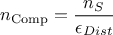
where  is the number of retained samples in the final posterior
distribution, as defined in the constructor (see Section XI.5.1).
is the number of retained samples in the final posterior
distribution, as defined in the constructor (see Section XI.5.1).
As previously explained, when comparing your reference dataset to a deterministic model (i.e., a model with
no intrinsic stochastic behaviour), the user can explicitly specify his own uncertainty assumptions. This
can be done by calling setGaussianNoise, whose prototype is
setGaussianNoise(stdname)
The idea is to inject random noise (assumed Gaussian and centered) into the model predictions, using internal
variables from the reference dataset to define its standard deviation. The only argument is a list of variables,
formatted as "stdvaria1:stdvaria2" , where each element corresponds to a variable within the reference
TDataServer. These values provide the standard deviation for each observation point (for example, to represent
experimental uncertainty).
This solution allows to:
define a common uncertainty (applied generally across all observations in the reference dataset) by simply adding an attribute with a
TAttributeFormula, where the formula is constant;use experimental uncertainties that are provided along with the reference values;
store all hypotheses within the reference
TDataServerobject. For this reason, we strongly recommend saving both the parameter and reference datasets at the end of a calibration procedure.
Warning
The number of variables in thestdname list must match the number of model outputs. Even in the
special case where calibration involves two outputs, with one having no associated uncertainty, a zero-valued
attribute should still be added for that output if the other requires an uncertainty model.
Finally, once the computation is complete (using the standard estimateParameters method),
the results can be examined in two main ways (in addition to inspecting the final datasets):
using the
drawParametersmethod, introduced in Section XI.2.3.6;using the
drawResidualsmethod, introduced in Section XI.2.3.7.
No additional options or visualization methods are specific to the TRejectionABC
implementation; these functions behave exactly as described in their respective sections.
An example is also provided in the use-case section (see Section XIV.12.4).
| |  | |
| XI.4. Analytical linear Bayesian estimation |  | XI.6. Markov chain Monte Carlo approach |