

Documentation
/ User's manual in Python
: 
| XIV.6. Macros Sensitivity | ||
|---|---|---|
 | Chapter XIV. Use-cases in python |  |
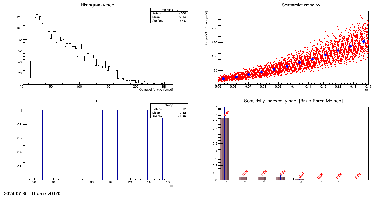
The objective of this macro is to perform a sensitivity analysis with brute force method on a set of eight parameters used in the flowrate model described in Section IV.1.2.1. Sensitivity indexes are computed dividing conditional variance by the standard deviation of the output variable.
Warning
This macro is purely illustrative. It is not meant to be used for proper results with a real code / function as it needs a large number of computation to only get the first order index. Its main appeal is to be nicely illustrative: it shows plainly the definition of the conditional expectation and also its variance used to defined the first order sobol indices."""
Example of Sobol estimation with a brut-force approach
"""
from rootlogon import ROOT, DataServer, Launcher, Sampler
def draw_bar_with_tuple(val, name, stitle):
"""Draw the results estimated with brut-force approach."""
h_div = ROOT.TH1F("hDivdrawBarWithTuple", stitle, 3, 0, 3)
h_div.SetCanExtend(ROOT.TH1.kXaxis) # .SetBit(ROOT.TH1.kCanRebin)
h_div.SetStats(0)
if h_div != 0:
h_div.SetBarWidth(0.45)
h_div.SetBarOffset(0.1)
h_div.SetMarkerColor(2)
h_div.SetMarkerSize(2)
h_div.SetFillColor(49)
h_div.SetTitle(stitle)
for ite, value in enumerate(val):
h_div.Fill(name[ite], value)
h_div.LabelsDeflate()
h_div.LabelsOption(">u")
h_div.SetMinimum(0.0)
h_div.SetMaximum(1.0)
ROOT.gStyle.SetPaintTextFormat("5.2f")
h_div.Draw("bar2, text45")
return h_div
nCond = 50
nbins = 10
# Create a DataServer.TDataServer
tds = DataServer.TDataServer()
print(" ******************************************************")
print(" ** sensitivityBrutForceMethodFlowrate nbins[%i] nCond[%i]" %
(nbins, nCond))
print(" **")
# Create a DataServer.TDataServer
tds = DataServer.TDataServer()
# Add the eight attributes of the study with uniform law
tds.addAttribute(DataServer.TUniformDistribution("rw", 0.05, 0.15))
tds.addAttribute(DataServer.TUniformDistribution("r", 100.0, 50000.0))
tds.addAttribute(DataServer.TUniformDistribution("tu", 63070.0, 115600.0))
tds.addAttribute(DataServer.TUniformDistribution("tl", 63.1, 116.0))
tds.addAttribute(DataServer.TUniformDistribution("hu", 990.0, 1110.0))
tds.addAttribute(DataServer.TUniformDistribution("hl", 700.0, 820.0))
tds.addAttribute(DataServer.TUniformDistribution("l", 1120.0, 1680.0))
tds.addAttribute(DataServer.TUniformDistribution("kw", 9855.0, 12045.0))
nvar = tds.getNAttributes()
print(" ** nX["+str(nvar)+"]")
nS = nbins*nvar*nCond
print(" ** nS["+str(nS)+"]")
# sam = Sampler.TSampling(tds, "lhs", nS)
sam = Sampler.TQMC(tds, "halton", nS)
sam.generateSample()
# Load the function
ROOT.gROOT.LoadMacro("UserFunctions.C")
# Create a TLauncherFunction from a TDataServer and an analytical function
# Rename the outpout attribute "ymod"
tlf = Launcher.TLauncherFunction(tds, "flowrateModel",
"rw:r:tu:tl:hu:hl:l:kw", "ymod")
# Evaluate the function on all the design of experiments
tlf.setDrawProgressBar(False)
tlf.run()
Canvas = ROOT.TCanvas("c1", "Graph for the Macro modeler", 5, 64, 1270, 667)
pad = ROOT.TPad("pad", "pad", 0, 0.03, 1, 1)
pad.Draw()
pad.Divide(2, 2)
pad.cd(1)
tds.computeStatistic("ymod")
tds.draw("ymod")
dstdy = tds.getAttribute("ymod").getStd()
svary = dstdy * dstdy
print(" ** ymod: std["+str(round(dstdy, 4))+"] vary["+str(round(svary, 1))+"]")
tds.getAttribute("ymod").setOutput()
ROOT.gStyle.SetOptStat(1)
valSobolCrt = []
sName = []
c = ROOT.TCanvas()
c.Divide(2)
c.cd(1)
for ivar in range(nvar):
print(" *****************************")
print(" *** "+str(tds.getAttribute(ivar).GetName()))
svar = tds.getAttribute(ivar).GetName()
if ivar == 0:
pad.cd(2)
else:
c.cd(1)
tds.drawProfile("ymod:"+svar, "", "nclass="+str(nbins))
hprofs = ROOT.gPad.GetPrimitive("Profile ymod:%s (Bin = %i )" %
(svar, nbins+2))
ntd = ROOT.TNtupleD("dd", "sjsjs", "i:x:m")
ntd.SetMarkerColor(ROOT.kBlue)
ntd.SetMarkerStyle(8)
nnbins = hprofs.GetNbinsX()
for i in range(1, nnbins+1):
ntd.Fill(i-1, hprofs.GetBinCenter(i), hprofs.GetBinContent(i))
tds.draw("ymod:"+svar)
ntd.Draw("m:x", "", "same")
if ivar == 0:
pad.cd(3)
else:
c.cd(2)
ntd.Draw("m")
htemp = ROOT.gPad.GetPrimitive("htemp")
dvarcond = htemp.GetRMS()
# Tempory ROOT.TTree for histogram
valSobolCrt.append(dvarcond*dvarcond / svary)
sName.append(svar)
print(" *** S1[ %s] Cond. Var.[%4.6g] -- [%1.6g]" %
(svar, dvarcond*dvarcond, valSobolCrt[-1]))
c.Modified()
c.Update()
c.SaveAs("SAFlowRateVersus"+svar+".png")
pad.cd(4)
hDiv = draw_bar_with_tuple(valSobolCrt, sName,
"Sensitivity Indexes: ymod [Brute-Force Method]")
Each parameter is related to the TDataServer as a TAttribute and obeys an uniform law on specific
interval:
tds = DataServer.TDataServer("tdsflowreate", "DataBase flowreate");
tds.addAttribute(DataServer.TUniformDistribution("rw", 0.05, 0.15));
tds.addAttribute(DataServer.TUniformDistribution("r", 100.0, 50000.0));
tds.addAttribute(DataServer.TUniformDistribution("tu", 63070.0, 115600.0));
tds.addAttribute(DataServer.TUniformDistribution("tl", 63.1, 116.0));
tds.addAttribute(DataServer.TUniformDistribution("hu", 990.0, 1110.0));
tds.addAttribute(DataServer.TUniformDistribution("hl", 700.0, 820.0));
tds.addAttribute(DataServer.TUniformDistribution("l", 1120.0, 1680.0));
tds.addAttribute(DataServer.TUniformDistribution("kw", 9855.0, 12045.0));
A design-of-experiments is built with a "Halton" method ( = 4000):
sam=Sampler.TQMC(tds, "halton", nS);
sam.generateSample();
The function flowrateModel is loaded from the macro UserFunctions.C (the
file can be found in ${URANIESYS}/share/uranie/macros):
ROOT.gROOT.LoadMacro("UserFunctions.C");
The flowrateModel model is applied on previous variables:
tlf=Launcher.TLauncherFunction(tds, "flowrateModel","rw:r:tu:tl:hu:hl:l:kw","ymod");
tlf.run();
Characteristic values for the output attribute are computed:
tds.computeStatistic("ymod");
Sensitivity indexes are computed in the for loop. Average value of output variable is computed on nbins+2=12 points for each input variable:
c.cd(1);
...
nnbins = hprofs.GetNbinsX();
for i in range(1,nnbins+1): ntd.Fill(i-1, hprofs.GetBinCenter(i), hprofs.GetBinContent(i));
The RMS value is obtained from the graphic of ymod versus the considered output variable and the sensitivity index is computed dividing the conditional variance value by the standard deviation of the output variable ymod.
c.cd(2);
ntd.Draw("m");
htemp = ROOT.gPad.GetPrimitive("htemp");
dvarcond = htemp.GetRMS();
valSobolCrt.append(dvarcond*dvarcond /svary);
Processing sensitivityBrutForceMethodFlowrate.py...

--- Uranie v4.11/0 --- Developed with ROOT (6.36.06)
                      Copyright (C) 2013-2026 CEA/DES
                      Contact: support-uranie@cea.fr
                      Date: Tue Feb 10, 2026

 ******************************************************
 ** sensitivityBrutForceMethodFlowrate nbins[10] nCond[50]
 **
 ** nX[8]
 ** nS[4000]
 ** ymod: std[45.6059] vary[2079.9]
 *****************************
 *** rw
 *** S1[ rw] Cond. Var.[1763.28] -- [0.847774]
Info in <TCanvas::Print>: png file SAFlowRateVersusrw.png has been created
 *****************************
 *** r
 *** S1[ r] Cond. Var.[0.0624988] -- [3.00489e-05]
Info in <TCanvas::Print>: png file SAFlowRateVersusr.png has been created
 *****************************
 *** tu
 *** S1[ tu] Cond. Var.[0.0886501] -- [4.26223e-05]
Info in <TCanvas::Print>: png file SAFlowRateVersustu.png has been created
 *****************************
 *** tl
 *** S1[ tl] Cond. Var.[0.0909604] -- [4.37331e-05]
Info in <TCanvas::Print>: png file SAFlowRateVersustl.png has been created
 *****************************
 *** hu
 *** S1[ hu] Cond. Var.[88.368] -- [0.0424867]
Info in <TCanvas::Print>: png file SAFlowRateVersushu.png has been created
 *****************************
 *** hl
 *** S1[ hl] Cond. Var.[88.2039] -- [0.0424078]
Info in <TCanvas::Print>: png file SAFlowRateVersushl.png has been created
 *****************************
 *** l
 *** S1[ l] Cond. Var.[84.9543] -- [0.0408454]
Info in <TCanvas::Print>: png file SAFlowRateVersusl.png has been created
 *****************************
 *** kw
 *** S1[ kw] Cond. Var.[20.8848] -- [0.0100413]
Info in <TCanvas::Print>: png file SAFlowRateVersuskw.png has been created
The objective of this macro is to compute the finite differences indexes on a function.
"""
Example of finite difference approach to the flowrate model
"""
from rootlogon import ROOT, DataServer, Sensitivity

# loading the flowrateModel function
ROOT.gROOT.LoadMacro("UserFunctions.C")

# Define the DataServer  and add the attributes (stochastic variables here)
tds = DataServer.TDataServer("tdsflowrate", "DataBase flowrate")
tds.addAttribute(DataServer.TUniformDistribution("rw", 0.05, 0.15))
tds.addAttribute(DataServer.TUniformDistribution("r", 100.0, 50000.0))
tds.addAttribute(DataServer.TUniformDistribution("tu", 63070.0, 115600.0))
tds.addAttribute(DataServer.TUniformDistribution("tl", 63.1, 116.0))
tds.addAttribute(DataServer.TUniformDistribution("hu", 990.0, 1110.0))
tds.addAttribute(DataServer.TUniformDistribution("hl", 700.0, 820.0))
tds.addAttribute(DataServer.TUniformDistribution("l", 1120.0, 1680.0))
tds.addAttribute(DataServer.TUniformDistribution("kw", 9855.0, 12045.0))

tds.getAttribute("rw").setDefaultValue(0.075)
tds.getAttribute("r").setDefaultValue(25000.0)
tds.getAttribute("tu").setDefaultValue(90000.0)
tds.getAttribute("tl").setDefaultValue(90.0)
tds.getAttribute("hu").setDefaultValue(1050.0)
tds.getAttribute("hl").setDefaultValue(760.0)
tds.getAttribute("l").setDefaultValue(1400.0)
tds.getAttribute("kw").setDefaultValue(10500.0)

# Create a TFiniteDifferences object
tfindef = Sensitivity.TFiniteDifferences(tds, "flowrateModel",
                                         "rw:r:tu:tl:hu:hl:l:kw",
                                         "flowrateModel", "steps=1%")
tfindef.setDrawProgressBar(False)
tfindef.computeIndexes()
matRes = tfindef.getSensitivityMatrix()
matRes.Print()
The function flowrateModel is loaded from the macro UserFunctions.C (the
file can be found in ${URANIESYS}/share/uranie/macros)
gROOT.LoadMacro("UserFunctions.C");
Each parameter is related to the TDataServer as a TAttribute and obeys an uniform law on specific interval:
tds = DataServer.TDataServer("tdsflowreate", "DataBase flowreate");
tds.addAttribute(DataServer.TUniformDistribution("rw", 0.05, 0.15));
tds.addAttribute(DataServer.TUniformDistribution("r", 100.0, 50000.0));
tds.addAttribute(DataServer.TUniformDistribution("tu", 63070.0, 115600.0));
tds.addAttribute(DataServer.TUniformDistribution("tl", 63.1, 116.0));
tds.addAttribute(DataServer.TUniformDistribution("hu", 990.0, 1110.0));
tds.addAttribute(DataServer.TUniformDistribution("hl", 700.0, 820.0));
tds.addAttribute(DataServer.TUniformDistribution("l", 1120.0, 1680.0));
tds.addAttribute(DataServer.TUniformDistribution("kw", 9855.0, 12045.0));
Each parameter gets a default value:
tds.getAttribute("rw").setDefaultValue(0.075);
tds.getAttribute("r").setDefaultValue(25000.0);
tds.getAttribute("tu").setDefaultValue(90000.0);
tds.getAttribute("tl").setDefaultValue(90.0);
tds.getAttribute("hu").setDefaultValue(1050.0);
tds.getAttribute("hl").setDefaultValue(760.0);
tds.getAttribute("l").setDefaultValue(1400.0);
tds.getAttribute("kw").setDefaultValue(10500.0);
To instantiate the TFiniteDifferences object, one uses the TDataServer, the name of the function,
the name of the output of the function, the names of the input variables separated by ":" and the option to specify
the sampling:
tfindef=Sensitivity.TFiniteDifferences(tds, "flowrateModel", "rw:r:tu:tl:hu:hl:l:kw", "flowrateModel", "steps=1%");
Computation of sensitivity indexes:
tfindef.computeIndexes();
Processing sensitivityFiniteDifferencesFunctionFlowrate.py...

--- Uranie v4.11/0 --- Developed with ROOT (6.36.06)
                      Copyright (C) 2013-2026 CEA/DES
                      Contact: support-uranie@cea.fr
                      Date: Tue Feb 10, 2026


1x8 matrix is as follows

     |      0    |      1    |      2    |      3    |      4    |
----------------------------------------------------------------------
   0 |       1019  -3.586e-07   1.265e-09    0.001265      0.1321


     |      5    |      6    |      7    |
----------------------------------------------------------------------
   0 |    -0.1321    -0.02729    0.003639
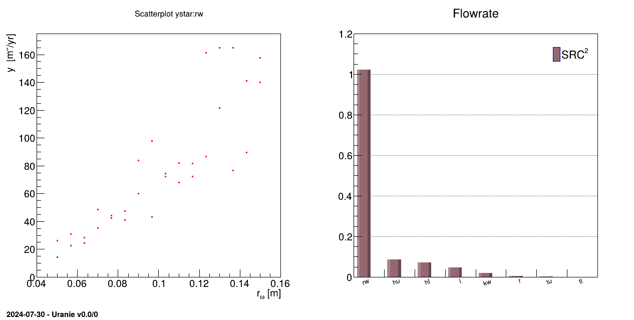
The objective of this macro is to perform a SRC regression on data stored in a TDataServer. Data are loaded in
the TDataServer from an ASCII data file flowrateUniformDesign.dat:
#NAME: flowrateborehole
#TITLE: Uniform design of flow rate borehole problem proposed by Ho and Xu(2000)
#COLUMN_NAMES: rw| r| tu| tl| hu| hl| l| kw | ystar
#COLUMN_TITLES: r_{#omega}| r | T_{u} | T_{l} | H_{u} | H_{l} | L | K_{#omega} | y^{*}
#COLUMN_UNITS: m | m | m^{2}/yr | m^{2}/yr | m | m | m | m/yr | m^{3}/yr

0.0500 33366.67  63070.0 116.00 1110.00 768.57 1200.0 11732.14  26.18
0.0500   100.00  80580.0  80.73 1092.86 802.86 1600.0 10167.86  14.46
0.0567   100.00  98090.0  80.73 1058.57 717.14 1680.0 11106.43  22.75
0.0567 33366.67  98090.0  98.37 1110.00 734.29 1280.0 10480.71  30.98
0.0633   100.00 115600.0  80.73 1075.71 751.43 1600.0 11106.43  28.33
0.0633 16733.33  80580.0  80.73 1058.57 785.71 1680.0 12045.00  24.60
0.0700 33366.67  63070.0  98.37 1092.86 768.57 1200.0 11732.14  48.65
0.0700 16733.33 115600.0 116.00  990.00 700.00 1360.0 10793.57  35.36
0.0767   100.0  115600.0  80.73 1075.71 751.43 1520.0 10793.57  42.44
0.0767 16733.33  80580.0  80.73 1075.71 802.86 1120.0  9855.00  44.16
0.0833 50000.00  98090.0  63.10 1041.43 717.14 1600.0 10793.57  47.49
0.0833 50000.00 115600.0  63.10 1007.14 768.57 1440.0 11419.29  41.04
0.0900 16733.33  63070.0 116.00 1075.71 751.43 1120.0 11419.29  83.77
0.0900 33366.67 115600.0 116.00 1007.14 717.14 1360.0 11106.43  60.05
0.0967 50000.00  80580.0  63.10 1024.29 820.00 1360.0  9855.00  43.15
0.0967 16733.33  80580.0  98.37 1058.57 700.00 1120.0 10480.71  97.98
0.1033 50000.00  80580.0  63.10 1024.29 700.00 1520.0 10480.71  74.44
0.1033 16733.33  80580.0  98.37 1058.57 820.00 1120.0 10167.86  72.23
0.1100 50000.00  98090.0  63.10 1024.29 717.14 1520.0 10793.57  82.18
0.1100   100.00  63070.0  98.37 1041.43 802.86 1600.0 12045.00  68.06
0.1167 33366.67  63070.0 116.00  990.00 785.71 1280.0 12045.00  81.63
0.1167   100.00  98090.0  98.37 1092.86 802.86 1680.0  9855.00  72.5
0.1233 16733.33 115600.0  80.73 1092.86 734.29 1200.0 11419.29 161.35
0.1233 16733.33  63070.0  63.10 1041.43 785.71 1680.0 12045.00  86.73
0.1300 33366.67  80580.0 116.00 1110.00 768.57 1280.0 11732.14 164.78
0.1300   100.00  98090.0  98.37 1110.00 820.00 1280.0 10167.86 121.76
0.1367 50000.00  98090.0  63.10 1007.14 820.00 1440.0 10167.86  76.51
0.1367 33366.67  98090.0 116.00 1024.29 700.00 1200.0 10480.71 164.75
0.1433 50000.00  63070.0 116.00  990.00 785.71 1440.0  9855.00  89.54
0.1433 50000.00 115600.0  63.10 1007.14 734.29 1440.0 11732.14 141.09
0.1500 33366.67  63070.0  98.37  990.00 751.43 1360.0 11419.29 139.94
0.1500   100.00 115600.0  80.73 1041.43 734.29 1520.0 11106.43 157.59
"""
Example of sensitivity analysis through linear regression
"""
from rootlogon import ROOT, DataServer, Sensitivity

# Create a DataServer.TDataServer
tds = DataServer.TDataServer()
# Load a database in an ASCII file
tds.fileDataRead("flowrateUniformDesign.dat")

# Graph
Canvas = ROOT.TCanvas("c2", "Graph for the Macro", 5, 64, 1270, 667)
# Visualisation
tds.Draw("ystar:rw")

# Sensitivity analysis
treg = Sensitivity.TRegression(tds, "rw:r:tu:tl:hu:hl:l:kw", "ystar", "src")
treg.computeIndexes()

treg.drawIndexes("Flowrate", "", "hist, first")
# treg.getResultTuple().Scan()

# Graph
c = ROOT.gROOT.FindObject("__sensitivitycan__0")
can = ROOT.TCanvas("c1", "Graph for the Macro sensitivityDataBaseFlowrate",
                   5, 64, 1270, 667)
pad = ROOT.TPad("pad", "pad", 0, 0.03, 1, 1)
pad.Draw()
pad.Divide(2)
pad.cd(1)
Canvas.DrawClonePad()
pad.cd(2)
c.DrawClonePad()
The TDataServer is filled with the data file flowrateUniformDesign.dat through the
fileDataRead method:
tds.fileDataRead("flowrateUniformDesign.dat");
The regression is performed on all the variables with a SRC method and sensitivity indexes are computed:
treg=Sensitivity.TRegression(tds, "rw:r:tu:tl:hu:hl:l:kw", "ystar", "src");
treg.computeIndexes();
The objective of this macro is to perform a Fast sensitivity analysis on a set of eight parameters used in the
flowrateModel model described in Section IV.1.2.1.
"""
Example of the flowrate function sensitivity analysis
"""
from rootlogon import ROOT, DataServer, Sensitivity

ROOT.gROOT.LoadMacro("UserFunctions.C")

# Define the DataServer
tds = DataServer.TDataServer("tdsflowreate", "DataBase flowreate")
tds.addAttribute(DataServer.TUniformDistribution("rw", 0.05, 0.15))
tds.addAttribute(DataServer.TUniformDistribution("r", 100.0, 50000.0))
tds.addAttribute(DataServer.TUniformDistribution("tu", 63070.0, 115600.0))
tds.addAttribute(DataServer.TUniformDistribution("tl", 63.1, 116.0))
tds.addAttribute(DataServer.TUniformDistribution("hu", 990.0, 1110.0))
tds.addAttribute(DataServer.TUniformDistribution("hl", 700.0, 820.0))
tds.addAttribute(DataServer.TUniformDistribution("l", 1120.0, 1680.0))
tds.addAttribute(DataServer.TUniformDistribution("kw", 9855.0, 12045.0))

# \param Size of a sampling.
nS = 4000
# Graph
fast = Sensitivity.TFast(tds, "flowrateModel", nS)
fast.setDrawProgressBar(False)
fast.computeIndexes("graph")

fast.getResultTuple().Scan("Out:Inp:Order:Method:Value", "Algo==\"--first--\"")
The function flowrateModel is loaded from the macro UserFunctions.C (the
file can be found in ${URANIESYS}/share/uranie/macros)
gROOT.LoadMacro("UserFunctions.C");
Each parameter is related to the TDataServer as a TAttribute and obeys an uniform law on specific interval:
tds = DataServer.TDataServer("tdsflowreate", "DataBase flowreate");
tds.addAttribute(DataServer.TUniformDistribution("rw", 0.05, 0.15));
tds.addAttribute(DataServer.TUniformDistribution("r", 100.0, 50000.0));
tds.addAttribute(DataServer.TUniformDistribution("tu", 63070.0, 115600.0));
tds.addAttribute(DataServer.TUniformDistribution("tl", 63.1, 116.0));
tds.addAttribute(DataServer.TUniformDistribution("hu", 990.0, 1110.0));
tds.addAttribute(DataServer.TUniformDistribution("hl", 700.0, 820.0));
tds.addAttribute(DataServer.TUniformDistribution("l", 1120.0, 1680.0));
tds.addAttribute(DataServer.TUniformDistribution("kw", 9855.0, 12045.0));
To instantiate the TFast object, one uses the TDataServer, the name of the function and the number
of samplings needed to perform sensitivity analysis (here nS=500):
tfast=Sensitivity.TFast(tds, "flowrateModel", nS);
Computation of sensitivity indexes:
tfast.computeIndexes();
Processing sensitivityFASTFunctionFlowrate.py...

--- Uranie v4.11/0 --- Developed with ROOT (6.36.06)
                      Copyright (C) 2013-2026 CEA/DES
                      Contact: support-uranie@cea.fr
                      Date: Tue Feb 10, 2026

 <URANIE::WARNING>
 <URANIE::WARNING> *** URANIE WARNING ***
 <URANIE::WARNING> *** File[${SOURCEDIR}/dataSERVER/souRCE/TDataServer.cxx] Line[8531]
 <URANIE::WARNING> TDataServer::getTuple Error : There is no tree!
 <URANIE::WARNING> *** END of URANIE WARNING ***
 <URANIE::WARNING>
 <URANIE::WARNING>
 <URANIE::WARNING> *** URANIE WARNING ***
 <URANIE::WARNING> *** File[${SOURCEDIR}/dataSERVER/souRCE/TDataServer.cxx] Line[8531]
 <URANIE::WARNING> TDataServer::getTuple Error : There is no tree!
 <URANIE::WARNING> *** END of URANIE WARNING ***
 <URANIE::WARNING>
 <URANIE::INFO>
 <URANIE::INFO> *** URANIE INFORMATION ***
 <URANIE::INFO> *** File[${SOURCEDIR}/meTIER/sampler/souRCE/TSpaceFilling.cxx] Line[167]
 <URANIE::INFO> TSamplerStochastic::init: the TDS [tdsflowreate] contains data: we need to empty it !
 <URANIE::INFO> *** END of URANIE INFORMATION ***
 <URANIE::INFO>
************************************************************************
*    Row   *       Out *       Inp *     Order *    Method *     Value *
************************************************************************
*        0 * flowrateM *        rw *     First *      FAST * 0.8278187 *
*        2 * flowrateM *         r *     First *      FAST * 8.924e-07 *
*        4 * flowrateM *        tu *     First *      FAST * 2.308e-06 *
*        6 * flowrateM *        tl *     First *      FAST * 3.204e-05 *
*        8 * flowrateM *        hu *     First *      FAST * 0.0414390 *
*       10 * flowrateM *        hl *     First *      FAST * 0.0414046 *
*       12 * flowrateM *         l *     First *      FAST * 0.0392873 *
*       14 * flowrateM *        kw *     First *      FAST * 0.0094983 *
************************************************************************
==> 8 selected entries
The objective of this macro is to perform a RBD sensitivity analysis on a set of eight parameters used in the
flowrateModel model described in Section IV.1.2.1.
"""
Example of RDB analysis on the flowrate function
"""
from rootlogon import ROOT, DataServer, Sensitivity

ROOT.gROOT.LoadMacro("UserFunctions.C")

# Define the DataServer
tds = DataServer.TDataServer("tdsflowrate", "DataBase flowrate")
tds.addAttribute(DataServer.TUniformDistribution("rw", 0.05, 0.15))
tds.addAttribute(DataServer.TUniformDistribution("r", 100.0, 50000.0))
tds.addAttribute(DataServer.TUniformDistribution("tu", 63070.0, 115600.0))
tds.addAttribute(DataServer.TUniformDistribution("tl", 63.1, 116.0))
tds.addAttribute(DataServer.TUniformDistribution("hu", 990.0, 1110.0))
tds.addAttribute(DataServer.TUniformDistribution("hl", 700.0, 820.0))
tds.addAttribute(DataServer.TUniformDistribution("l", 1120.0, 1680.0))
tds.addAttribute(DataServer.TUniformDistribution("kw", 9855.0, 12045.0))

# Size of a sampling.
nS = 4000
# Graph
trbd = Sensitivity.TRBD(tds, "flowrateModel", nS)
trbd.setDrawProgressBar(False)
trbd.computeIndexes("graph")

trbd.getResultTuple().Scan("Out:Inp:Order:Method:Value", "Algo==\"--first--\"")
The function flowrateModel is loaded from the macro UserFunctions.C
(the file can be found in ${URANIESYS}/share/uranie/macros)
gROOT.LoadMacro("UserFunctions.C");
Each parameter is related to the TDataServer as a TAttribute and obeys an uniform law on specific
interval
tds = DataServer.TDataServer("tdsflowreate", "DataBase flowreate");
tds.addAttribute(DataServer.TUniformDistribution("rw", 0.05, 0.15));
tds.addAttribute(DataServer.TUniformDistribution("r", 100.0, 50000.0));
tds.addAttribute(DataServer.TUniformDistribution("tu", 63070.0, 115600.0));
tds.addAttribute(DataServer.TUniformDistribution("tl", 63.1, 116.0));
tds.addAttribute(DataServer.TUniformDistribution("hu", 990.0, 1110.0));
tds.addAttribute(DataServer.TUniformDistribution("hl", 700.0, 820.0));
tds.addAttribute(DataServer.TUniformDistribution("l", 1120.0, 1680.0));
tds.addAttribute(DataServer.TUniformDistribution("kw", 9855.0, 12045.0));
To instantiate the TRBD object, one uses the TDataServer, the name of the function and the number
of samplings needed to perform sensitivity analysis (here =4000):
trbd=Sensitivity.TRBD(tds, "flowrateModel", nS);
Computation of sensitivity indexes:
trbd.computeIndexes();
Processing sensitivityRBDFunctionFlowrate.py...

--- Uranie v4.11/0 --- Developed with ROOT (6.36.06)
                      Copyright (C) 2013-2026 CEA/DES
                      Contact: support-uranie@cea.fr
                      Date: Tue Feb 10, 2026

 <URANIE::WARNING>
 <URANIE::WARNING> *** URANIE WARNING ***
 <URANIE::WARNING> *** File[${SOURCEDIR}/dataSERVER/souRCE/TDataServer.cxx] Line[8531]
 <URANIE::WARNING> TDataServer::getTuple Error : There is no tree!
 <URANIE::WARNING> *** END of URANIE WARNING ***
 <URANIE::WARNING>
 <URANIE::WARNING>
 <URANIE::WARNING> *** URANIE WARNING ***
 <URANIE::WARNING> *** File[${SOURCEDIR}/dataSERVER/souRCE/TDataServer.cxx] Line[8531]
 <URANIE::WARNING> TDataServer::getTuple Error : There is no tree!
 <URANIE::WARNING> *** END of URANIE WARNING ***
 <URANIE::WARNING>
 <URANIE::INFO>
 <URANIE::INFO> *** URANIE INFORMATION ***
 <URANIE::INFO> *** File[${SOURCEDIR}/meTIER/sampler/souRCE/TSpaceFilling.cxx] Line[167]
 <URANIE::INFO> TSamplerStochastic::init: the TDS [tdsflowrate] contains data: we need to empty it !
 <URANIE::INFO> *** END of URANIE INFORMATION ***
 <URANIE::INFO>
************************************************************************
*    Row   *       Out *       Inp *     Order *    Method *     Value *
************************************************************************
*        0 * flowrateM *        rw *     First *       RBD * 0.7558010 *
*        2 * flowrateM *         r *     First *       RBD * 0.0026080 *
*        4 * flowrateM *        tu *     First *       RBD * 0.0035324 *
*        6 * flowrateM *        tl *     First *       RBD * 0.0032848 *
*        8 * flowrateM *        hu *     First *       RBD * 0.0408758 *
*       10 * flowrateM *        hl *     First *       RBD * 0.0469345 *
*       12 * flowrateM *         l *     First *       RBD * 0.0347870 *
*       14 * flowrateM *        kw *     First *       RBD * 0.0165843 *
************************************************************************
==> 8 selected entries
The objective of this macro is to perform a Morris sensitivity analysis on a set of eight parameters used in the
flowrateModel model described in Section IV.1.2.1.
"""
Example of Morris estimation on flowrate
"""
from rootlogon import ROOT, DataServer, Sensitivity

ROOT.gROOT.LoadMacro("UserFunctions.C")

# Define the DataServer
tds = DataServer.TDataServer("tdsflowreate", "DataBase flowreate")

tds.addAttribute(DataServer.TUniformDistribution("rw", 0.05, 0.15))
tds.addAttribute(DataServer.TUniformDistribution("r", 100.0, 50000.0))
tds.addAttribute(DataServer.TUniformDistribution("tu", 63070.0, 115600.0))
tds.addAttribute(DataServer.TUniformDistribution("tl", 63.1, 116.0))
tds.addAttribute(DataServer.TUniformDistribution("hu", 990.0, 1110.0))
tds.addAttribute(DataServer.TUniformDistribution("hl", 700.0, 820.0))
tds.addAttribute(DataServer.TUniformDistribution("l", 1120.0, 1680.0))
tds.addAttribute(DataServer.TUniformDistribution("kw", 9855.0, 12045.0))

nreplique = 3
nlevel = 10
scmo = Sensitivity.TMorris(tds, "flowrateModel", nreplique, nlevel)
scmo.setDrawProgressBar(False)
scmo.generateSample()

tds.exportData("_morris_sampling_.dat")
scmo.computeIndexes()

tds.exportData("_morris_launching_.dat")

ntresu = scmo.getMorrisResults()
ntresu.Scan("*")

# Graph
canmoralltraj = ROOT.gROOT.FindObject("canmoralltraj")
can = ROOT.TCanvas("c1", "Graph of sensitivityMorrisFunctionFlowrate",
                   5, 64, 1270, 667)
pad = ROOT.TPad("pad", "pad", 0, 0.03, 1, 1)
pad.Draw()
pad.Divide(2)
pad.cd(1)
scmo.drawSample("", -1, "nonewcanv")
pad.cd(2)
scmo.drawIndexes("mustar", "", "nonewcanv")
The function flowrateModel is loaded from the macro UserFunctions.C
(the file can be found in ${URANIESYS}/share/uranie/macros)
gROOT.LoadMacro("UserFunctions.C");
Each parameter is related to the TDataServer as a TAttribute and obeys an uniform law on specific
interval:
tds = DataServer.TDataServer("tdsflowreate", "DataBase flowreate");
tds.addAttribute(DataServer.TUniformDistribution("rw", 0.05, 0.15));
tds.addAttribute(DataServer.TUniformDistribution("r", 100.0, 50000.0));
tds.addAttribute(DataServer.TUniformDistribution("tu", 63070.0, 115600.0));
tds.addAttribute(DataServer.TUniformDistribution("tl", 63.1, 116.0));
tds.addAttribute(DataServer.TUniformDistribution("hu", 990.0, 1110.0));
tds.addAttribute(DataServer.TUniformDistribution("hl", 700.0, 820.0));
tds.addAttribute(DataServer.TUniformDistribution("l", 1120.0, 1680.0));
tds.addAttribute(DataServer.TUniformDistribution("kw", 9855.0, 12045.0));
To instantiate the TMorris , one uses the TDataServer, the name of the function, the number of
replicas (here nreplique=3), the level parameter (here nlevel=10)
scmo=Sensitivity.TMorris(tds, "flowrateModel", nreplique, nlevel);
Creation of the sampling:
scmo.generateSample();
Data are exported in an ASCII file:
tds.exportData("_morris_sampling_.dat");
Computation of sensitivity indexes:
scmo.computeIndexes();
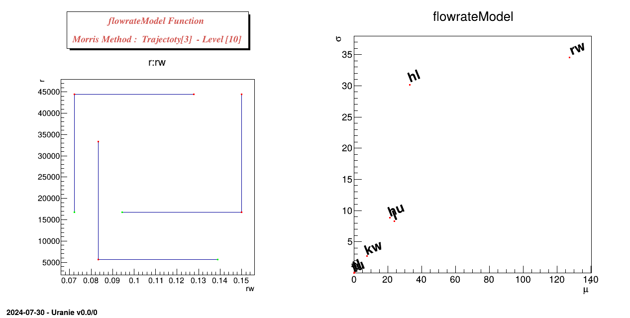
Processing sensitivityMorrisFunctionFlowrate.py...
************************************************************************
*    Row   *     Input *    Output *     mu.mu * mustar.mu * sigma.sig *
************************************************************************
*        0 *        rw * flowrateM * 127.47900 * 127.47900 * 34.521839 *
*        1 *         r * flowrateM * -0.069601 * 0.0696013 * 0.0793689 *
*        2 *        tu * flowrateM * 0.0004201 * 0.0004201 * 0.0004641 *
*        3 *        tl * flowrateM * 0.4659763 * 0.4659763 * 0.3301256 *
*        4 *        hu * flowrateM * 21.192361 * 21.192361 * 8.8498989 *
*        5 *        hl * flowrateM * -32.74887 * 32.748874 * 30.146134 *
*        6 *         l * flowrateM * -23.89328 * 23.893280 * 8.2781934 *
*        7 *        kw * flowrateM * 7.5766167 * 7.5766167 * 2.7457665 *
************************************************************************
The objective of this macro is to perform a Morris sensitivity analysis on a set of eight parameters used in the
flowrateModel model described in Section IV.1.2.1, but this time using the Relauncher architecture.
"""
Example of Morris analysis on flowrate with a Relauncher approach
"""
from rootlogon import ROOT, DataServer, Relauncher, Sensitivity

ROOT.gROOT.LoadMacro("UserFunctions.C")

# Define the DataServer
rw = DataServer.TUniformDistribution("rw", 0.05, 0.15)
r = DataServer.TUniformDistribution("r", 100.0, 50000.0)
tu = DataServer.TUniformDistribution("tu", 63070.0, 115600.0)
tl = DataServer.TUniformDistribution("tl", 63.1, 116.0)
hu = DataServer.TUniformDistribution("hu", 990.0, 1110.0)
hl = DataServer.TUniformDistribution("hl", 700.0, 820.0)
lvar = DataServer.TUniformDistribution("l", 1120.0, 1680.0)
kw = DataServer.TUniformDistribution("kw", 9855.0, 12045.0)

# Create the evaluator
code = Relauncher.TCIntEval("flowrateModel")
# Create output attribute
yout = DataServer.TAttribute("flowrateModel")
# Provide input/output attributes to the assessor
code.addInput(rw)
code.addInput(r)
code.addInput(tu)
code.addInput(tl)
code.addInput(hu)
code.addInput(hl)
code.addInput(lvar)
code.addInput(kw)
code.addOutput(yout)

run = Relauncher.TSequentialRun(code)  # Replace to distribute computation
run.startSlave()
if run.onMaster():
    # Create the dataserver
    tds = DataServer.TDataServer("sobol", "foo bar pouet chocolat")
    tds.addAttribute(rw)
    tds.addAttribute(r)
    tds.addAttribute(tu)
    tds.addAttribute(tl)
    tds.addAttribute(hu)
    tds.addAttribute(hl)
    tds.addAttribute(lvar)
    tds.addAttribute(kw)

    # Create the Morris object
    nreplique = 3
    nlevel = 10
    scmo = Sensitivity.TMorris(tds, run, nreplique, nlevel)
    scmo.setDrawProgressBar(False)
    scmo.generateSample()

    tds.exportData("_morris_sampling_.dat")
    scmo.computeIndexes()

    tds.exportData("_morris_launching_.dat")

    ntresu = scmo.getMorrisResults()
    ntresu.Scan("*")

    # Graph
    canmoralltraj = ROOT.gROOT.FindObject("canmoralltraj")
    can = ROOT.TCanvas("c1", "Graph sensitivityMorrisFunctionFlowrateRunner",
                       5, 64, 1270, 667)
    pad = ROOT.TPad("pad", "pad", 0, 0.03, 1, 1)
    pad.Draw()
    pad.Divide(2)
    pad.cd(1)
    scmo.drawSample("", -1, "nonewcanv")
    pad.cd(2)
    scmo.drawIndexes("mustar", "", "nonewcanv")
The function flowrateModel is loaded from the macro UserFunctions.C
(the file can be found in ${URANIESYS}/share/uranie/macros)
ROOT.gROOT.LoadMacro("UserFunctions.C");
Each parameter is related to the TDataServer as a TAttribute and obeys an uniform law on specific
interval:
# Define the DataServer
rw=DataServer.TUniformDistribution("rw", 0.05, 0.15);
r=DataServer.TUniformDistribution("r", 100.0, 50000.0);
tu=DataServer.TUniformDistribution("tu", 63070.0, 115600.0);
tl=DataServer.TUniformDistribution("tl", 63.1, 116.0);
hu=DataServer.TUniformDistribution("hu", 990.0, 1110.0);
hl=DataServer.TUniformDistribution("hl", 700.0, 820.0);
l=DataServer.TUniformDistribution("l", 1120.0, 1680.0);
kw=DataServer.TUniformDistribution("kw", 9855.0, 12045.0);
The interface to the function is then defined, using the Relauncher interface, through a
TCIntEval object and a sequential runner. On the contrary to the C++ script, python cannot
use methods such as setInputs or setOutputs and the inputs and
outputs have to be included ony-by-one.
# Create the evaluator
code=Relauncher.TCIntEval("flowrateModel");
# Create output attribute
yout=DataServer.TAttribute("flowrateModel");
# Provide input/output attributes to the assessor
code.addInput(rw)
code.addInput(r)
code.addInput(tu)
code.addInput(tl)
code.addInput(hu)
code.addInput(hl)
code.addInput(l)
code.addInput(kw);
code.addOutput(yout);

run=Relauncher.TSequentialRun(code); # To be replaced to distribute the computation
run.startSlave();
The dataserver object is defined only on the master to avoid useless replication if one wants to run the estimation
of the function in parallel (by changing the TSequentialRun by either a
TThreadedRun or a TMpiRun). To instantiate the
TMorris object, one uses the TDataServer, a pointer to the chosen runner, the number of replicas
(here nreplique=3), the level parameter (here nlevel=10)
scmo=Sensitivity.TMorris(tds, run, nreplique, nlevel);
Creation of the sampling:
scmo.generateSample();
Data are exported in an ASCII file:
tds.exportData("_morris_sampling_.dat");
Computation of sensitivity indexes:
scmo.computeIndexes();The rest of the code is providing command to get a final plot.

Processing sensitivityMorrisFunctionFlowrateRunner.py...
************************************************************************
*    Row   *     Input *    Output *     mu.mu * mustar.mu * sigma.sig *
************************************************************************
*        0 *        rw * flowrateM * 127.47900 * 127.47900 * 34.521839 *
*        1 *         r * flowrateM * -0.069601 * 0.0696013 * 0.0793689 *
*        2 *        tu * flowrateM * 0.0004201 * 0.0004201 * 0.0004641 *
*        3 *        tl * flowrateM * 0.4659763 * 0.4659763 * 0.3301256 *
*        4 *        hu * flowrateM * 21.192361 * 21.192361 * 8.8498989 *
*        5 *        hl * flowrateM * -32.74887 * 32.748874 * 30.146134 *
*        6 *         l * flowrateM * -23.89328 * 23.893280 * 8.2781934 *
*        7 *        kw * flowrateM * 7.5766167 * 7.5766167 * 2.7457665 *
************************************************************************
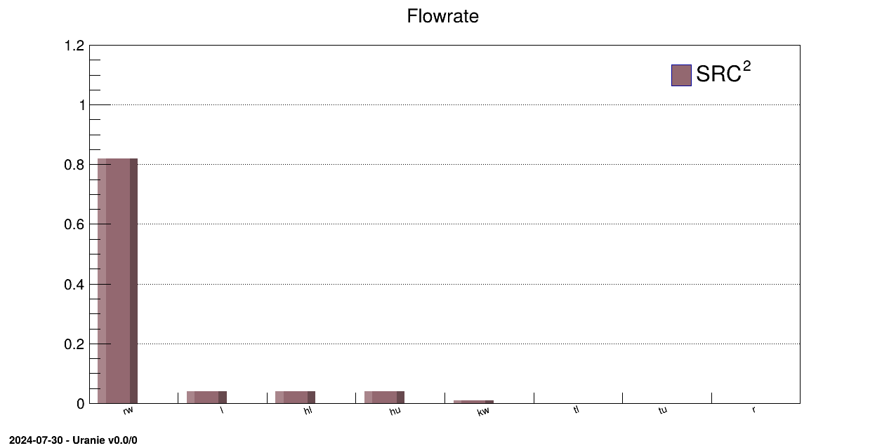
The objective of this macro is to perform a regression with "SRC" method on a database generated with a function
using sampling of parameters obeying uniform laws with 4000 patterns. flowrateModel is a
function defined in Section IV.1.2.1 and "loaded" through the
macro UserFunctions.C (the file can be found in
${URANIESYS}/share/uranie/macros). Function flowrateModel uses the eight
variables defined in Section IV.1.2.1 and set in the main macro.
"""
Example of regression approach on the flowrate function
"""
from rootlogon import ROOT, DataServer, Launcher, Sampler, Sensitivity

ROOT.gROOT.LoadMacro("UserFunctions.C")

# Define the DataServer
tds = DataServer.TDataServer("tdsflowreate", "DataBase flowreate")
tds.addAttribute(DataServer.TUniformDistribution("rw", 0.05, 0.15))
tds.addAttribute(DataServer.TUniformDistribution("r", 100.0, 50000.0))
tds.addAttribute(DataServer.TUniformDistribution("tu", 63070.0, 115600.0))
tds.addAttribute(DataServer.TUniformDistribution("tl", 63.1, 116.0))
tds.addAttribute(DataServer.TUniformDistribution("hu", 990.0, 1110.0))
tds.addAttribute(DataServer.TUniformDistribution("hl", 700.0, 820.0))
tds.addAttribute(DataServer.TUniformDistribution("l", 1120.0, 1680.0))
tds.addAttribute(DataServer.TUniformDistribution("kw", 9855.0, 12045.0))

# Size of a sampling.
nS = 4000

sampling = Sampler.TSampling(tds, "lhs", nS)
sampling.generateSample()

tlf = Launcher.TLauncherFunction(tds, "flowrateModel")
tlf.setDrawProgressBar(False)
tlf.run()

treg = Sensitivity.TRegression(tds, "rw:r:tu:tl:hu:hl:l:kw",
                               "flowrateModel", "SRC")
treg.computeIndexes()
treg.getResultTuple().SetScanField(60)

treg.getResultTuple().Scan("Out:Inp:Method:Algo:Value:CILower:CIUpper",
                           "Order==\"First\"")

can = ROOT.TCanvas("c1", "Graph sensitivityRegressionFunctionFlowrate",
                   5, 64, 1270, 667)
treg.drawIndexes("Flowrate", "", "hist, first, nonewcanv")
Each attribute is related to a TAttribute obeying uniform laws on specific intervals:
tds.addAttribute(DataServer.TUniformDistribution("rw", 0.05, 0.15));
tds.addAttribute(DataServer.TUniformDistribution("r", 100.0, 50000.0));
tds.addAttribute(DataServer.TUniformDistribution("tu", 63070.0, 115600.0));
tds.addAttribute(DataServer.TUniformDistribution("tl", 63.1, 116.0));
tds.addAttribute(DataServer.TUniformDistribution("hu", 990.0, 1110.0));
tds.addAttribute(DataServer.TUniformDistribution("hl", 700.0, 820.0));
tds.addAttribute(DataServer.TUniformDistribution("l", 1120.0, 1680.0));
tds.addAttribute(DataServer.TUniformDistribution("kw", 9855.0, 12045.0));
The sampling is generated on 4000 patterns with a LHS method:
sampling = Sampler.TSampling(tds, "lhs", 4000);
sampling.generateSample();
Function flowrateModel is set to perform calculation on the sampling:
tlf=Launcher.TLauncherFunction(tds, "flowrateModel");
tlf.run();
The regression is performed over all variables:
treg=Sensitivity.TRegression(tds, "rw:r:tu:tl:hu:hl:l:kw","flowrateModel", "SRC");
treg.computeIndexes();
Sensitivity indexes are then displayed through an histogram and a pie graph:
can=ROOT.TCanvas("c1", "Graph for the Macro sensitivityRegressionFunctionFlowrate",5,64,1270,667);
treg.drawIndexes("Flowrate", "", "hist,first,nonewcanv");
Processing sensitivityRegressionFunctionFlowrate.py...

--- Uranie v4.11/0 --- Developed with ROOT (6.36.06)
                      Copyright (C) 2013-2026 CEA/DES
                      Contact: support-uranie@cea.fr
                      Date: Tue Feb 10, 2026

*************************************************************************************
*    Row   *    Out *      Inp * Metho *      Algo *    Value *  CILower *  CIUpper *
*************************************************************************************
*        0 * flowra *       rw * SRC^2 * --first-- * 0.820265 *       -1 *       -1 *
*        2 * flowra *       rw * SRC^2 * --rho^2-- *  0.81668 * 0.805846 * 0.826888 *
*        4 * flowra *        r * SRC^2 * --first-- * 5.97e-06 *       -1 *       -1 *
*        6 * flowra *        r * SRC^2 * --rho^2-- * 1.92e-06 * 2.65e-07 * 0.001339 *
*        8 * flowra *       tu * SRC^2 * --first-- * 8.64e-06 *       -1 *       -1 *
*       10 * flowra *       tu * SRC^2 * --rho^2-- * 4.03e-06 * 3.14e-07 * 0.001306 *
*       12 * flowra *       tl * SRC^2 * --first-- * 5.73e-05 *       -1 *       -1 *
*       14 * flowra *       tl * SRC^2 * --rho^2-- * 0.000209 * 7.34e-07 * 0.002085 *
*       16 * flowra *       hu * SRC^2 * --first-- * 0.039645 *       -1 *       -1 *
*       18 * flowra *       hu * SRC^2 * --rho^2-- * 0.037119 * 0.026221 * 0.049000 *
*       20 * flowra *       hl * SRC^2 * --first-- * 0.040597 *       -1 *       -1 *
*       22 * flowra *       hl * SRC^2 * --rho^2-- * 0.039708 * 0.028688 * 0.052470 *
*       24 * flowra *        l * SRC^2 * --first-- * 0.040895 *       -1 *       -1 *
*       26 * flowra *        l * SRC^2 * --rho^2-- * 0.041241 * 0.029896 * 0.054454 *
*       28 * flowra *       kw * SRC^2 * --first-- * 0.009174 *       -1 *       -1 *
*       30 * flowra *       kw * SRC^2 * --rho^2-- * 0.009090 * 0.004191 * 0.015767 *
*       32 * flowra *  __sum__ * SRC^2 * --first-- *  0.95065 *       -1 *       -1 *
*       34 * flowra *   __R2__ * SRC^2 * --first-- * 0.947296 *       -1 *       -1 *
*       36 * flowra *  __R2A__ * SRC^2 * --first-- *  0.94719 *       -1 *       -1 *
*************************************************************************************
==> 19 selected entries
The objective of this macro is to perform Sobol sensitivity analysis on a set of eight parameters used in the
flowrateModel model described in Section IV.1.2.1.
"""
Example of Sobol estimation for the flowrate function
"""
from rootlogon import ROOT, DataServer, Sensitivity
ROOT.gROOT.LoadMacro("UserFunctions.C")
# Define the DataServer
tds = DataServer.TDataServer("tdsflowreate", "DataBase flowreate")
tds.addAttribute(DataServer.TUniformDistribution("rw", 0.05, 0.15))
tds.addAttribute(DataServer.TUniformDistribution("r", 100.0, 50000.0))
tds.addAttribute(DataServer.TUniformDistribution("tu", 63070.0, 115600.0))
tds.addAttribute(DataServer.TUniformDistribution("tl", 63.1, 116.0))
tds.addAttribute(DataServer.TUniformDistribution("hu", 990.0, 1110.0))
tds.addAttribute(DataServer.TUniformDistribution("hl", 700.0, 820.0))
tds.addAttribute(DataServer.TUniformDistribution("l", 1120.0, 1680.0))
tds.addAttribute(DataServer.TUniformDistribution("kw", 9855.0, 12045.0))
ns = 100000
tsobol = Sensitivity.TSobol(tds, "flowrateModel", ns, "rw:r:tu:tl:hu:hl:l:kw",
"flowrateModel", "DummyPython")
tsobol.setDrawProgressBar(False)
tsobol.computeIndexes()
tsobol.getResultTuple().Scan("*", "Algo==\"--first--\" || Algo==\"--total--\"")
cc = ROOT.TCanvas("c1", "histgramme", 5, 64, 1270, 667)
pad = ROOT.TPad("pad", "pad", 0, 0.03, 1, 1)
pad.Draw()
pad.Divide(2, 1)
pad.cd(1)
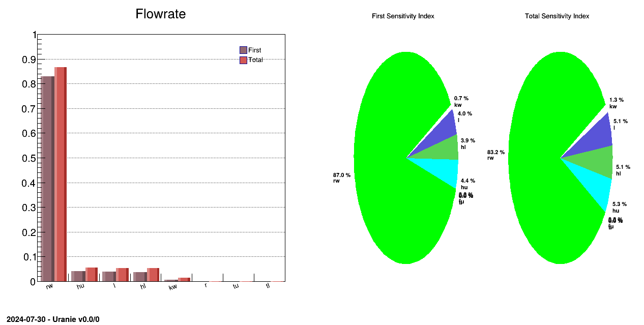
tsobol.drawIndexes("Flowrate", "", "nonewcanv, hist, all")
pad.cd(2)
tsobol.drawIndexes("Flowrate", "", "nonewcanv, pie, first")
ROOT.gSystem.Rename("_sobol_launching_.dat", "ref_sobol_launching_.dat")
tds.exportData("_onlyMandN_sobol_launching_.dat",
"rw:r:tu:tl:hu:hl:l:kw:flowrateModel",
"sobol__n__iter__tdsflowreate < 100")
The function flowrateModel is loaded from the macro UserFunctions.C (the
file can be found in ${URANIESYS}/share/uranie/macros)
gROOT.LoadMacro("UserFunctions.C");
Each parameter is related to the TDataServer as a TAttribute and obeys an uniform law on specific interval:
tds = DataServer.TDataServer("tdsflowreate", "DataBase flowreate");
tds.addAttribute(DataServer.TUniformDistribution("rw", 0.05, 0.15));
tds.addAttribute(DataServer.TUniformDistribution("r", 100.0, 50000.0));
tds.addAttribute(DataServer.TUniformDistribution("tu", 63070.0, 115600.0));
tds.addAttribute(DataServer.TUniformDistribution("tl", 63.1, 116.0));
tds.addAttribute(DataServer.TUniformDistribution("hu", 990.0, 1110.0));
tds.addAttribute(DataServer.TUniformDistribution("hl", 700.0, 820.0));
tds.addAttribute(DataServer.TUniformDistribution("l", 1120.0, 1680.0));
tds.addAttribute(DataServer.TUniformDistribution("kw", 9855.0, 12045.0));
To instantiate the TSobol, one uses the TDataServer, the name of the function and the number of samplings
needed to perform sensitivity analysis (here ns=600):
tsobol=Sensitivity.TSobol(tds, "flowrateModel", ns, "rw:r:tu:tl:hu:hl:l:kw", "flowrateModel", "DummyPython");
The last argument is the option field, which in most cases is empty. Here it is filled with "DummyPython" which
helps specify to python which constructor to choose. There are indeed several possible constructors these 5 five
first arguments, but C++ can make the difference between them as the literal members are either
std::string, ROOT::TString, Char_t* or even Option_t*. For
python, these format are all PyString, so the sixth argument is compulsory to disentangle the
possibilities.
Computation of the sensitivity indexes:
tsobol.computeIndexes();
Data are exported from the TDataServer to an ASCII file:
tds.exportData("_sobol_launching_.dat");

Processing sensitivitySobolFunctionFlowrate.py...

--- Uranie v4.11/0 --- Developed with ROOT (6.36.06)
                      Copyright (C) 2013-2026 CEA/DES
                      Contact: support-uranie@cea.fr
                      Date: Tue Feb 10, 2026

 <URANIE::WARNING>
 <URANIE::WARNING> *** URANIE WARNING ***
 <URANIE::WARNING> *** File[${SOURCEDIR}/dataSERVER/souRCE/TDataServer.cxx] Line[8531]
 <URANIE::WARNING> TDataServer::getTuple Error : There is no tree!
 <URANIE::WARNING> *** END of URANIE WARNING ***
 <URANIE::WARNING>
 <URANIE::INFO>
 <URANIE::INFO> *** URANIE INFORMATION ***
 <URANIE::INFO> *** File[${SOURCEDIR}/meTIER/sampler/souRCE/TSamplerStochastic.cxx] Line[66]
 <URANIE::INFO> TSamplerStochastic::init: the TDS [tdsflowreate] contains data: we need to empty it !
 <URANIE::INFO> *** END of URANIE INFORMATION ***
 <URANIE::INFO>
 ** Case of Output atty [flowrateModel]  nSimPerIndex 10000
 ** Input att [rw] First [0.830033] Total Order[0.865762]
 ** Input att [r] First [0] Total Order[0.000102212]
 ** Input att [tu] First [0] Total Order[0.0001]
 ** Input att [tl] First [0] Total Order[0.000110756]
 ** Input att [hu] First [0.0417298] Total Order[0.0554922]
 ** Input att [hl] First [0.0367345] Total Order[0.0526188]
 ** Input att [l] First [0.0384214] Total Order[0.0535728]
 ** Input att [kw] First [0.00669831] Total Order[0.0132316]
************************************************************************************************************
*    Row   *   Out.Out *   Inp.Inp * Order.Ord * Method.Me * Algo.Algo * Value.Val * CILower.C * CIUpper.C *
************************************************************************************************************
*        0 * flowrateM *        rw *     First *     Sobol * --first-- * 0.8300331 * 0.8238356 * 0.8360321 *
*        4 * flowrateM *        rw *     Total *     Sobol * --total-- * 0.8657619 * 0.8465652 * 0.8850599 *
*        8 * flowrateM *         r *     First *     Sobol * --first-- *         0 *         0 * 0.0196004 *
*       12 * flowrateM *         r *     Total *     Sobol * --total-- * 0.0001022 * 9.828e-05 * 0.0001062 *
*       16 * flowrateM *        tu *     First *     Sobol * --first-- *         0 *         0 * 0.0196004 *
*       20 * flowrateM *        tu *     Total *     Sobol * --total-- * 0.0001000 * 9.615e-05 * 0.0001039 *
*       24 * flowrateM *        tl *     First *     Sobol * --first-- *         0 *         0 * 0.0196004 *
*       28 * flowrateM *        tl *     Total *     Sobol * --total-- * 0.0001107 * 0.0001064 * 0.0001151 *
*       32 * flowrateM *        hu *     First *     Sobol * --first-- * 0.0417297 * 0.0221474 * 0.0612800 *
*       36 * flowrateM *        hu *     Total *     Sobol * --total-- * 0.0554921 * 0.0534156 * 0.0576470 *
*       40 * flowrateM *        hl *     First *     Sobol * --first-- * 0.0367345 * 0.0171464 * 0.0562944 *
*       44 * flowrateM *        hl *     Total *     Sobol * --total-- * 0.0526187 * 0.0506469 * 0.0546652 *
*       48 * flowrateM *         l *     First *     Sobol * --first-- * 0.0384214 * 0.0188352 * 0.0579782 *
*       52 * flowrateM *         l *     Total *     Sobol * --total-- * 0.0535727 * 0.0515661 * 0.0556552 *
*       56 * flowrateM *        kw *     First *     Sobol * --first-- * 0.0066983 *         0 * 0.0262952 *
*       60 * flowrateM *        kw *     Total *     Sobol * --total-- * 0.0132315 * 0.0127261 * 0.0137570 *
*       64 * flowrateM *   __sum__ *     First *     Sobol * --first-- * 0.9536171 *        -1 *        -1 *
*       65 * flowrateM *   __sum__ *     Total *     Sobol * --total-- * 1.0409902 *        -1 *        -1 *
************************************************************************************************************
==> 18 selected entries
The objective of this macro is to perform Sobol sensitivity analysis on a set of eight parameters used in the
flowrateModel model described in Section IV.1.2.1, but this time using the Relauncher architecture.
"""
Example of Sobol estimation for the flowrate function with Relauncher approach
"""
from rootlogon import ROOT, DataServer, Relauncher, Sensitivity

ROOT.gROOT.LoadMacro("UserFunctions.C")

# Define the DataServer
rw = DataServer.TUniformDistribution("rw", 0.05, 0.15)
r = DataServer.TUniformDistribution("r", 100.0, 50000.0)
tu = DataServer.TUniformDistribution("tu", 63070.0, 115600.0)
tl = DataServer.TUniformDistribution("tl", 63.1, 116.0)
hu = DataServer.TUniformDistribution("hu", 990.0, 1110.0)
hl = DataServer.TUniformDistribution("hl", 700.0, 820.0)
lvar = DataServer.TUniformDistribution("l", 1120.0, 1680.0)
kw = DataServer.TUniformDistribution("kw", 9855.0, 12045.0)

# Create the evaluator
code = Relauncher.TCIntEval("flowrateModel")
# Create output attribute
yout = DataServer.TAttribute("flowrateModel")
# Provide input/output attributes to the assessor
code.addInput(rw)
code.addInput(r)
code.addInput(tu)
code.addInput(tl)
code.addInput(hu)
code.addInput(hl)
code.addInput(lvar)
code.addInput(kw)
code.addOutput(yout)

run = Relauncher.TSequentialRun(code)  # Replace to distribute computation
run.startSlave()
if run.onMaster():
    # Create the dataserver
    tds = DataServer.TDataServer("sobol", "foo bar pouet chocolat")
    code.addAllInputs(tds)

    # Create the sobol object
    ns = 100000
    tsobol = Sensitivity.TSobol(tds, run, ns)
    tsobol.setDrawProgressBar(ROOT.kFALSE)
    tsobol.computeIndexes()

    cc = ROOT.TCanvas("c1", "histgramme", 5, 64, 1270, 667)
    pad = ROOT.TPad("pad", "pad", 0, 0.03, 1, 1)
    pad.Draw()
    pad.Divide(2, 1)
    pad.cd(1)
    tsobol.drawIndexes("Flowrate", "", "nonewcanv, hist, all")

    pad.cd(2)
    tsobol.drawIndexes("Flowrate", "", "nonewcanv, pie, first")
The function flowrateModel is loaded from the macro UserFunctions.C (the
file can be found in ${URANIESYS}/share/uranie/macros)
ROOT.gROOT.LoadMacro("UserFunctions.C");
Each parameter is related to the TDataServer as a TAttribute and obeys an uniform law on specific interval:
# Define the DataServer
rw=DataServer.TUniformDistribution("rw", 0.05, 0.15);
r=DataServer.TUniformDistribution("r", 100.0, 50000.0);
tu=DataServer.TUniformDistribution("tu", 63070.0, 115600.0);
tl=DataServer.TUniformDistribution("tl", 63.1, 116.0);
hu=DataServer.TUniformDistribution("hu", 990.0, 1110.0);
hl=DataServer.TUniformDistribution("hl", 700.0, 820.0);
l=DataServer.TUniformDistribution("l", 1120.0, 1680.0);
kw=DataServer.TUniformDistribution("kw", 9855.0, 12045.0);
The interface to the function is then defined, using the Relauncher interface, through a
TCIntEval object and a sequential runner:
# Create the evaluator
code=Relauncher.TCIntEval("flowrateModel");
# Create output attribute
yout=DataServer.TAttribute("flowrateModel");
# Provide input/output attributes to the assessor
code.addInput(rw)
code.addInput(r)
code.addInput(tu)
code.addInput(tl)
code.addInput(hu)
code.addInput(hl)
code.addInput(l)
code.addInput(kw);
code.addOutput(yout);

run=Relauncher.TSequentialRun(code); # To be replaced to distribute the computation
run.startSlave();
To instantiate the TSobol, one uses the TDataServer, a pointer to the runner and the number of
samplings needed to perform sensitivity analysis (here ns=600):
tsobol = Sensitivity.TSobol(tds, run, ns);
Computation of the sensitivity indexes:
tsobol.computeIndexes();
Data are exported from the TDataServer to an ASCII file:
tds.exportData("_sobol_launching_.dat");

Processing sensitivitySobolFunctionFlowrateRunner.py...

--- Uranie v4.11/0 --- Developed with ROOT (6.36.06)
                      Copyright (C) 2013-2026 CEA/DES
                      Contact: support-uranie@cea.fr
                      Date: Tue Feb 10, 2026

 <URANIE::WARNING>
 <URANIE::WARNING> *** URANIE WARNING ***
 <URANIE::WARNING> *** File[${SOURCEDIR}/dataSERVER/souRCE/TDataServer.cxx] Line[8531]
 <URANIE::WARNING> TDataServer::getTuple Error : There is no tree!
 <URANIE::WARNING> *** END of URANIE WARNING ***
 <URANIE::WARNING>
 <URANIE::INFO>
 <URANIE::INFO> *** URANIE INFORMATION ***
 <URANIE::INFO> *** File[${SOURCEDIR}/meTIER/sampler/souRCE/TSamplerStochastic.cxx] Line[66]
 <URANIE::INFO> TSamplerStochastic::init: the TDS [sobol] contains data: we need to empty it !
 <URANIE::INFO> *** END of URANIE INFORMATION ***
 <URANIE::INFO>
 ** Case of Output atty [flowrateModel]  nSimPerIndex 10000
 ** Input att [rw] First [0.830033] Total Order[0.865762]
 ** Input att [r] First [0] Total Order[0.000102212]
 ** Input att [tu] First [0] Total Order[0.0001]
 ** Input att [tl] First [0] Total Order[0.000110756]
 ** Input att [hu] First [0.0417298] Total Order[0.0554922]
 ** Input att [hl] First [0.0367345] Total Order[0.0526188]
 ** Input att [l] First [0.0384214] Total Order[0.0535728]
 ** Input att [kw] First [0.00669831] Total Order[0.0132316]
Warning
The levele command will be installed on your machine only if a Fortran compiler is found
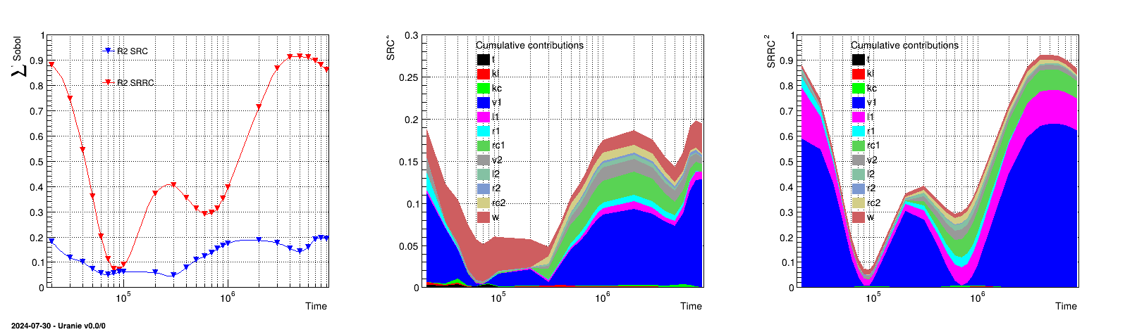
The objective of this macro is to perform a SRC and SRRC measurement on the temporal use-case levele. This use-case is an example of code that takes a dozen of entries in order to compute the evolution of dose as a function of time. The result of every computation consists in 3 vectors: the time (always the same value disregarding all entries), the dose called "y" and a third useless information.
"""
Example of regression analysis on the levelE code
"""
import sys
from ctypes import c_double  # for ROOT version greater or equal to 6.20
import numpy as np
from rootlogon import ROOT, Launcher, Sampler, Sensitivity
from rootlogon import DataServer as DS

# Exit if levele not found
if ROOT.gSystem.Exec("which levele"):
    sys.exit(-1)

# Create DataServer and add input attributes
tds = DS.TDataServer("tds", "levelE usecase")
tds.addAttribute(DS.TUniformDistribution("t", 100, 1000))
tds.addAttribute(DS.TLogUniformDistribution("kl", 0.001, .01))
tds.addAttribute(DS.TLogUniformDistribution("kc", 1.0e-6, 1.0e-5))
tds.addAttribute(DS.TLogUniformDistribution("v1", 1.0e-3, 1.0e-1))
tds.addAttribute(DS.TUniformDistribution("l1", 100., 500.))
tds.addAttribute(DS.TUniformDistribution("r1", 1., 5.))
tds.addAttribute(DS.TUniformDistribution("rc1", 3., 30.))
tds.addAttribute(DS.TLogUniformDistribution("v2", 1.0e-2, 1.0e-1))
tds.addAttribute(DS.TUniformDistribution("l2", 50., 200.))
tds.addAttribute(DS.TUniformDistribution("r2", 1., 5.))
tds.addAttribute(DS.TUniformDistribution("rc2", 3., 30.))
tds.addAttribute(DS.TLogUniformDistribution("w", 1.0e5, 1.0e7))

# Tell the code where to find attribute value in input file
sIn = "levelE_input_with_values_rows.in"
tds.getAttribute("t").setFileKey(sIn, "", "%e", DS.TAttributeFileKey.kNewRow)
tds.getAttribute("kl").setFileKey(sIn, "", "%e", DS.TAttributeFileKey.kNewRow)
tds.getAttribute("kc").setFileKey(sIn, "", "%e", DS.TAttributeFileKey.kNewRow)
tds.getAttribute("v1").setFileKey(sIn, "", "%e", DS.TAttributeFileKey.kNewRow)
tds.getAttribute("l1").setFileKey(sIn, "", "%e", DS.TAttributeFileKey.kNewRow)
tds.getAttribute("r1").setFileKey(sIn, "", "%e", DS.TAttributeFileKey.kNewRow)
tds.getAttribute("rc1").setFileKey(sIn, "", "%e", DS.TAttributeFileKey.kNewRow)
tds.getAttribute("v2").setFileKey(sIn, "", "%e", DS.TAttributeFileKey.kNewRow)
tds.getAttribute("l2").setFileKey(sIn, "", "%e", DS.TAttributeFileKey.kNewRow)
tds.getAttribute("r2").setFileKey(sIn, "", "%e", DS.TAttributeFileKey.kNewRow)
tds.getAttribute("rc2").setFileKey(sIn, "", "%e", DS.TAttributeFileKey.kNewRow)
tds.getAttribute("w").setFileKey(sIn, "", "%e", DS.TAttributeFileKey.kNewRow)

# Create DOE
ns = 1024
samp = Sampler.TSampling(tds, "lhs", ns)
samp.generateSample()

# How to read ouput files
out = Launcher.TOutputFileRow("_output_levelE_withRow_.dat")
# Tell the output file that attribute IS a vector and is SECOND column
out.addAttribute(DS.TAttribute("y", DS.TAttribute.kVector), 2)

# Creation of Launcher.TCode
myc = Launcher.TCode(tds, " levele 2> /dev/null")
myc.addOutputFile(out)

# Run the code
tl = Launcher.TLauncher(tds, myc)
tl.run()

# Launch Regression
tsen = Sensitivity.TRegression(tds, "t:kl:kc:v1:l1:r1:rc1:v2:l2:r2:rc2:w",
                               "y", "SRCSRRC")
tsen.computeIndexes()
res = tsen.getResultTuple()

# Plotting mess
tps = np.array([20000, 30000, 40000, 50000, 60000, 70000, 80000, 90000, 100000,
                200000, 300000, 400000, 500000, 600000, 700000, 800000, 900000,
                1e+06, 2e+06, 3e+06, 4e+06, 5e+06, 6e+06, 7e+06, 8e+06, 9e+06],
               dtype=float)
colors = [1, 2, 3, 4, 6, 7, 8, 15, 30, 38, 41, 46]

c2 = ROOT.TCanvas("c2", "c2", 5, 64, 1600, 500)
pad = ROOT.TPad("pad", "pad", 0, 0.03, 1, 1)
pad.Draw()
pad.Divide(3, 1)
pad.cd(1)
ROOT.gPad.SetLogx()
ROOT.gPad.SetGrid()
mg = ROOT.TMultiGraph()
res.Draw("Value", "Inp==\"__R2__\" && Order==\"Total\" && Method==\"SRRC^2\"",
         "goff")
data3 = res.GetV1()

gr3 = ROOT.TGraph(26, tps, data3)
gr3.SetMarkerColor(2)
gr3.SetLineColor(2)
gr3.SetMarkerStyle(23)
mg.Add(gr3)
res.Draw("Value", "Inp==\"__R2__\" && Order==\"Total\" && Method==\"SRC^2\"",
         "goff")
data4 = res.GetV1()

gr4 = ROOT.TGraph(26, tps, data4)
gr4.SetMarkerColor(4)
gr4.SetLineColor(4)
gr4.SetMarkerStyle(23)
mg.Add(gr4)
mg.Draw("APC")
mg.GetXaxis().SetTitle("Time")
mg.GetYaxis().SetTitle("#sum Sobol")
mg.GetYaxis().SetRangeUser(0.0, 1.0)

# Legend
ROOT.gStyle.SetLegendBorderSize(0)
ROOT.gStyle.SetFillStyle(0)

lg = ROOT.TLegend(0.25, 0.7, 0.45, 0.9)
lg.AddEntry(gr4, "R2 SRC", "lp")
lg.AddEntry(gr3, "R2 SRRC", "lp")
lg.Draw()


pad.cd(2)
ROOT.gPad.SetLogx()
ROOT.gPad.SetGrid()
mg2 = ROOT.TMultiGraph()

names = ["t", "kl", "kc", "v1", "l1", "r1", "rc1",
         "v2", "l2", "r2", "rc2", "w"]
src = [0, 0, 0, 0, 0, 0, 0, 0, 0, 0, 0, 0]
leg = ROOT.TLegend(0.25, 0.3, 0.45, 0.89, "Cumulative contributions")
leg.SetTextSize(0.035)
for igr in range(12):

    sel = "Inp==\""+names[igr]+"\""
    sel += "&& Order==\"Total\" && Method==\"SRC^2\" && Algo!=\"--rho^2--\""
    res.Draw("Value", sel, "goff")
    data = res.GetV1()
    src[igr] = ROOT.TGraph()
    src[igr].SetMarkerColor(colors[igr])
    src[igr].SetLineColor(colors[igr])
    src[igr].SetFillColor(colors[igr])

    src[igr].SetPoint(0, 0.99999999*tps[0], 0)
    for ip in range(26):

        x = c_double(0)
        y = c_double(0)  # For ROOT lower than 6.20, user ROOT.Double
        if igr != 0:
            src[igr-1].GetPoint(ip+1, x, y)
        src[igr].SetPoint(ip+1, tps[ip], y.value+data[ip])

    src[igr].SetPoint(27, tps[25]*1.000000001, 0)
    leg.AddEntry(src[igr], names[igr], "f")

for igr2 in range(11, -1, -1):
    mg2.Add(src[igr2])

mg2.Draw("AFL")
mg2.GetXaxis().SetTitle("Time")
mg2.GetYaxis().SetTitle("SRC^{2}")
mg2.GetYaxis().SetRangeUser(0.0, 0.3)
leg.Draw()

pad.cd(3)
ROOT.gPad.SetLogx()
ROOT.gPad.SetGrid()
mg3 = ROOT.TMultiGraph()
srrc = [0, 0, 0, 0, 0, 0, 0, 0, 0, 0, 0, 0]

for igr in range(12):
    sel = "Inp==\""+names[igr]+"\""
    sel += "&& Order==\"Total\" && Method==\"SRRC^2\" && Algo!=\"--rho^2--\""
    res.Draw("Value", sel, "goff")
    data = res.GetV1()
    srrc[igr] = ROOT.TGraph()
    srrc[igr].SetMarkerColor(colors[igr])
    srrc[igr].SetLineColor(colors[igr])
    srrc[igr].SetFillColor(colors[igr])

    srrc[igr].SetPoint(0, 0.99999999*tps[0], 0)
    for ip in range(26):
        x = c_double(0)
        y = c_double(0)  # For ROOT lower than 6.20, user ROOT.Double
        if igr != 0:
            srrc[igr-1].GetPoint(ip+1, x, y)
        srrc[igr].SetPoint(ip+1, tps[ip], y.value+data[ip])

    srrc[igr].SetPoint(27, tps[25]*1.000000001, 0)
    srrc[igr].SetTitle(names[igr])

for igr2 in range(11, -1, -1):
    mg3.Add(srrc[igr2])

# mg3.Draw("a fb l3d")
mg3.Draw("AFL")
mg3.GetXaxis().SetTitle("Time")
mg3.GetYaxis().SetTitle("SRRC^{2}")
mg3.GetYaxis().SetRangeUser(0.0, 1.0)
leg.Draw()
The levele external code is located in the bin directory of the Uranie installation.
When looking at the code and comparing it to an usual Regression estimation, the organisation is completely transparent. The only noticeable (and compulsory) thing to do is to change the default type of the attribute read at the end of the job. This is done in this line:
out.addAttribute(DataServer.TAttribute("y", DataServer.TAttribute.kVector), 2 );
where the output attribute is provided, changing its nature to a vector, thanks to the second argument of the
TAttribute constructor from the default (kReal) to the desired
nature (kVector). Once this is done, this information is broadcast internally to the code
that knows how to deal with this type of attribute.
The rest of the code is the graphical part, leading to the figure below (it is provided to illustrate how to represent results).
The results of the previous macro is shown in Figure XIV.54, where the left panel represents the value of the
 coefficients both the SRC
and SRRC coefficients estimation. The middle and right panel display the cumulative sum of the quadratic value of
the coefficient respectively for the SRC and SRRC case.
coefficients both the SRC
and SRRC coefficients estimation. The middle and right panel display the cumulative sum of the quadratic value of
the coefficient respectively for the SRC and SRRC case.
Warning
The levele command will be installed on your machine only if a Fortran compiler is found
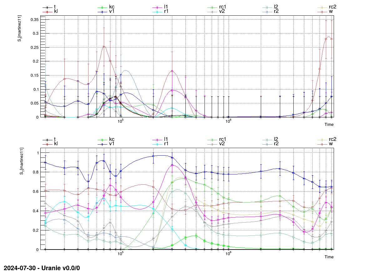
The objective of this macro is to perform a full Sobol analysis on the temporal use-case levele. This use-case is an example of code that takes a dozen of entries in order to compute the evolution of dose as a function of time. The result of every computation consists in 3 vectors: the time (always the same value disregarding all entries), the dose called "y" and a third useless information.
"""
Example of Sobol estimation on the levelE code
"""
import sys
import numpy as np
from rootlogon import ROOT, Launcher, Sensitivity
from rootlogon import DataServer as DS

# Exit if levele not found
if ROOT.gSystem.Exec("which levele"):
    sys.exit(-1)

# Define the DataServer
tds = DS.TDataServer("tdsLevelE", "levele")
tds.addAttribute(DS.TUniformDistribution("t", 100, 1000))
tds.addAttribute(DS.TLogUniformDistribution("kl", 0.001, 0.01))
tds.addAttribute(DS.TLogUniformDistribution("kc", 0.000001, 0.00001))
tds.addAttribute(DS.TLogUniformDistribution("v1", 0.001, 0.1))
tds.addAttribute(DS.TUniformDistribution("l1", 100, 500))
tds.addAttribute(DS.TUniformDistribution("r1", 1, 5))
tds.addAttribute(DS.TUniformDistribution("rc1", 3, 30))
tds.addAttribute(DS.TLogUniformDistribution("v2", 0.01, 0.1))
tds.addAttribute(DS.TUniformDistribution("l2", 50, 200))
tds.addAttribute(DS.TUniformDistribution("r2", 1, 5))
tds.addAttribute(DS.TUniformDistribution("rc2", 3, 30))
tds.addAttribute(DS.TLogUniformDistribution("w", 100000, 10000000))

# Tell the code where to find attribute value in input file
sIn = "levelE_input_with_values_rows.in"
tds.getAttribute("t").setFileKey(sIn, "", "%e", DS.TAttributeFileKey.kNewRow)
tds.getAttribute("kl").setFileKey(sIn, "", "%e", DS.TAttributeFileKey.kNewRow)
tds.getAttribute("kc").setFileKey(sIn, "", "%e", DS.TAttributeFileKey.kNewRow)
tds.getAttribute("v1").setFileKey(sIn, "", "%e", DS.TAttributeFileKey.kNewRow)
tds.getAttribute("l1").setFileKey(sIn, "", "%e", DS.TAttributeFileKey.kNewRow)
tds.getAttribute("r1").setFileKey(sIn, "", "%e", DS.TAttributeFileKey.kNewRow)
tds.getAttribute("rc1").setFileKey(sIn, "", "%e", DS.TAttributeFileKey.kNewRow)
tds.getAttribute("v2").setFileKey(sIn, "", "%e", DS.TAttributeFileKey.kNewRow)
tds.getAttribute("l2").setFileKey(sIn, "", "%e", DS.TAttributeFileKey.kNewRow)
tds.getAttribute("r2").setFileKey(sIn, "", "%e", DS.TAttributeFileKey.kNewRow)
tds.getAttribute("rc2").setFileKey(sIn, "", "%e", DS.TAttributeFileKey.kNewRow)
tds.getAttribute("w").setFileKey(sIn, "", "%e", DS.TAttributeFileKey.kNewRow)

# How to read ouput files
out = Launcher.TOutputFileRow("_output_levelE_withRow_.dat")
# Tell the output file that attribute IS a vector and is SECOND column
out.addAttribute(DS.TAttribute("y", DS.TAttribute.kVector), 2)

# Creation of Launcher.TCode
myc = Launcher.TCode(tds, "levele 2> /dev/null")
myc.addOutputFile(out)

# Run Sobol analysis
tsobol = Sensitivity.TSobol(tds, myc, 10000)
tsobol.computeIndexes()

ntresu = tsobol.getResultTuple()

# Plotting mess
colors = [1, 2, 3, 4, 6, 7, 8, 15, 30, 38, 41, 46]
tps = np.array([20000, 30000, 40000, 50000, 60000, 70000, 80000, 90000, 100000,
                200000, 300000, 400000, 500000, 600000, 700000, 800000, 900000,
                1e+06, 2e+06, 3e+06, 4e+06, 5e+06, 6e+06, 7e+06, 8e+06, 9e+06],
               dtype=float)

c2 = ROOT.TCanvas("c2", "c2", 5, 64, 1200, 900)
pad = ROOT.TPad("pad", "pad", 0, 0.03, 1, 1)
pad.Draw()
pad.Divide(1, 2)
pad.cd(1)
ROOT.gPad.SetLogx()
ROOT.gPad.SetGrid()

# LegendandMArker
ROOT.gStyle.SetMarkerStyle(3)
ROOT.gStyle.SetLegendBorderSize(0)
ROOT.gStyle.SetFillStyle(0)

mg2 = ROOT.TMultiGraph()
names = ["t", "kl", "kc", "v1", "l1", "r1", "rc1",
         "v2", "l2", "r2", "rc2", "w"]
fdeg = [0., 0., 0., 0., 0., 0., 0., 0., 0., 0., 0., 0.]
leg = [0., 0., 0., 0., 0., 0.]
Zeros = np.zeros([26])

for igr in range(12):

    sel = "Inp==\""+names[igr]+"\""
    sel += " && Order==\"First\" &&  Algo==\"martinez11\""
    ntresu.Draw("CILower:CIUpper:Value", sel, "goff")
    data = ntresu.GetV3()
    themin = ntresu.GetV1()
    themax = ntresu.GetV2()
    for i in range(26):
        themin[i] = data[i] - themin[i]
        themax[i] = - data[i] + themax[i]

    if (igr % 2) == 0:
        leg[int(igr/2)] = ROOT.TLegend(0.1+0.15*(igr/2), 0.91,
                                       0.25+0.15*(igr/2), 0.98)
        leg[int(igr/2)].SetTextSize(0.045)

    fdeg[igr] = ROOT.TGraphAsymmErrors(26, tps, data,
                                       Zeros, Zeros, themin, themax)
    fdeg[igr].SetMarkerColor(colors[igr])
    fdeg[igr].SetLineColor(colors[igr])
    fdeg[igr].SetFillColor(colors[igr])
    leg[int(igr/2)].AddEntry(fdeg[igr], names[igr], "pl")

for igr2 in range(11, -1, -1):
    mg2.Add(fdeg[igr2])

mg2.Draw("APC")
mg2.GetXaxis().SetTitle("Time")
mg2.GetYaxis().SetTitle("S_{1}[martinez11]")
for igr3 in range(6):
    leg[igr3].Draw()

mg = ROOT.TMultiGraph()
tdeg = [0., 0., 0., 0., 0., 0., 0., 0., 0., 0., 0., 0.]
pad.cd(2)
ROOT.gPad.SetLogx()
ROOT.gPad.SetGrid()
for igr in range(12):

    sel = "Inp==\""+names[igr]+"\""
    sel += " && Order==\"Total\" &&  Algo==\"martinez11\""
    ntresu.Draw("CILower:CIUpper:Value", sel, "goff")
    data = ntresu.GetV3()
    themin = ntresu.GetV1()
    themax = ntresu.GetV2()
    for i in range(26):
        themin[i] = data[i] - themin[i]
        themax[i] = - data[i] + themax[i]

    for ip in range(26):
        if ip == 0:
            tdeg[igr] = ROOT.TGraphAsymmErrors()
            tdeg[igr].SetMarkerColor(colors[igr])
            tdeg[igr].SetLineColor(colors[igr])
            tdeg[igr].SetFillColor(colors[igr])

        tdeg[igr].SetPoint(ip, tps[ip], data[ip])
        tdeg[igr].SetPointError(ip, 0, 0, themin[ip], themax[ip])

for igr2 in range(11, -1, -1):
    mg.Add(tdeg[igr2])

mg.Draw("APC")
mg.GetXaxis().SetTitle("Time")
mg.GetYaxis().SetTitle("S_{T}[martinez11]")
for igr3 in range(6):
    leg[igr3].Draw()
The levele external code is located in the bin directory of the Uranie installation.
When looking at the code and comparing it to an usual Sobol estimation, the organisation is completely transparent. The only noticeable (and compulsory) thing to do is to change the default type of the attribute read at the end of the job. This is done in this line:
out.addAttribute(DataServer.TAttribute("y", DataServer.TAttribute.kVector), 2 );
where the output attribute is provided, changing its nature to a vector, thanks to the second argument of the
TAttribute constructor from the default (kReal) to the desired
nature (kVector). Once this is done, this information is broadcast internally to the code
that knows how to deal with this type of attribute.
The rest of the code is the graphical part, leading to the figure below (it is provided to illustrate how to represent results).
The results of the previous macro is shown in Figure XIV.55, where the evolution of the sobol coefficient is shown for all inputs with the uncertainty band, for the first order coefficient and the total one, respectively on the top and bottom panel.
The objective of this macro is to perform a full Sobol analysis using the existing file created when the Sobol class is allowed to perform the design-of-experiments and the estimations by itself (see the first item in the tip box in Section VI.5.2 for more details). This would mean that the only computation done would be to estimate the coefficients (no external code / function called).
Warning
Theref_sobol_launching_.dat file used as input is not provided in the usual sub-directory
"/share/uranie/macros" of the installation folder of Uranie
($URANIESYS) but can be generated by the user by running the macro discussed in Section XIV.6.9.
"""
Example of sobol re-estimation
"""
from rootlogon import ROOT, DataServer, Sensitivity

ROOT.gROOT.LoadMacro("UserFunctions.C")

# Define the DataServer
tds = DataServer.TDataServer("tdsflowreate", "DataBase flowreate")
tds.fileDataRead("ref_sobol_launching_.dat")

tsobol = Sensitivity.TSobol(tds, "rw:r:tu:tl:hu:hl:l:kw", "flowrateModel")
tsobol.setDrawProgressBar(False)
tsobol.computeIndexes()

cc = ROOT.TCanvas("c1", "histgramme", 5, 64, 1270, 667)
pad = ROOT.TPad("pad", "pad", 0, 0.03, 1, 1)
pad.Draw()
pad.Divide(2, 1)
pad.cd(1)
tsobol.drawIndexes("Flowrate", "", "nonewcanv, hist, all")

pad.cd(2)
tsobol.drawIndexes("Flowrate", "", "nonewcanv, pie, first")
There are no external code or function to be run here. The input file ref_sobol_launching_.dat
has to be generated by the use of sensitivtySobolFunctionFlowrate.py. Once done it is loaded
into the dataserver and the TSobol object is constructed from the simplest constructor with
only the pointer to the dataserver, the input and output list:
tsobol=Sensitivity.TSobol(tds, "rw:r:tu:tl:hu:hl:l:kw", "flowrateModel")
Once done, the computeIndexes() method is called and few lines are shown to display the
results in the classical plot form, leading to the figure below (it is provided to illustrate how to represent
results). The numerical results are shown in the console below and are identical to the ones shown in Section XIV.6.9.4 from where the full sample is coming from.
The results of the previous macro is shown in Figure XIV.56, where the evolution of the sobol coefficient is shown for all inputs with the uncertainty band, for the first order coefficient and the total one, respectively on the top and bottom panel.
Processing sensitivitySobolRe-estimation.py...

--- Uranie v4.11/0 --- Developed with ROOT (6.36.06)
                      Copyright (C) 2013-2026 CEA/DES
                      Contact: support-uranie@cea.fr
                      Date: Tue Feb 10, 2026

 ** Case of Output atty [flowrateModel]  nSimPerIndex 10000
 ** Input att [rw] First [0.830033] Total Order[0.865762]
 ** Input att [r] First [0] Total Order[0.000102212]
 ** Input att [tu] First [0] Total Order[0.0001]
 ** Input att [tl] First [0] Total Order[0.000110756]
 ** Input att [hu] First [0.0417298] Total Order[0.0554922]
 ** Input att [hl] First [0.0367345] Total Order[0.0526188]
 ** Input att [l] First [0.0384214] Total Order[0.0535728]
 ** Input att [kw] First [0.00669831] Total Order[0.0132316]
The objective of this macro is to perform a Sobol analysis using the some already made computations in order to be
able to save ressources. The idea (discussed in the second item in the tip box in Section VI.5.2 is
indeed to use the provided points as the  first estimations corresponding to both the
  and
and  matrices content. The class will still have to create all the cross
configurations (the
matrices content. The class will still have to create all the cross
configurations (the  matrices) and launch their corresponding estimations. In order to do that there are few things to keep in mind:
The input file (here
_onlyMandN_sobol_launching_.dat) should contains input and output variables only, the user being in charge of having a decent design-of-experiments for the sobol estimation.
Warning
The_onlyMandN_sobol_launching_.dat file used as input is not provided in the usual sub-directory
"/share/uranie/macros" of the installation folder of Uranie
($URANIESYS) but can be generated by the user by running the macro discussed in Section XIV.6.9.
"""
Example of sobol estimation using provided data
"""
from rootlogon import ROOT, DataServer, Sensitivity

ROOT.gROOT.LoadMacro("UserFunctions.C")
# Define the DataServer
tds = DataServer.TDataServer("tdsflowreate", "DataBase flowrate")
tds.fileDataRead("_onlyMandN_sobol_launching_.dat")

ns = 10000
tsobol = Sensitivity.TSobol(tds, "flowrateModel", ns, "rw:r:tu:tl:hu:hl:l:kw",
                            "flowrateModel", "WithData")
tsobol.setDrawProgressBar(False)
tsobol.computeIndexes()

cc = ROOT.TCanvas("c1", "histgramme", 5, 64, 1270, 667)
pad = ROOT.TPad("pad", "pad", 0, 0.03, 1, 1)
pad.Draw()
pad.Divide(2, 1)
pad.cd(1)
tsobol.drawIndexes("Flowrate", "", "nonewcanv, hist, all")

pad.cd(2)
tsobol.drawIndexes("Flowrate", "", "nonewcanv, pie, first")
As for Section XIV.6.9, the UserFunctions.C file
is loaded and the input file _onlyMandN_sobol_launching_.dat (which should have been
generated by the use of sensitivtySobolFunctionFlowrate.py), is loaded into the
dataserver. The TSobol object is constructed from the usual function constructor with a
noticing difference: the option field is filled with WithData to specify that data are
already there and the code has to use these data and split them into both the and matrices.
tsobol=Sensitivity.TSobol(tds, "flowrateModel", ns, "rw:r:tu:tl:hu:hl:l:kw", "flowrateModel", "WithData")
Once done, the computeIndexes() method is called and few lines are shown to display the
results in the classical plot form, leading to the figure below (it is provided to illustrate how to represent
results). The numerical results are shown in the console below and are identical to the ones shown in Section XIV.6.9.4 from where the original set of points is coming from.
The results of the previous macro is shown in Figure XIV.57, where the evolution of the sobol coefficient is shown for all inputs with the uncertainty band, for the first order coefficient and the total one, respectively on the top and bottom panel.

Processing sensitivitySobolWithData.py...

--- Uranie v4.11/0 --- Developed with ROOT (6.36.06)
                      Copyright (C) 2013-2026 CEA/DES
                      Contact: support-uranie@cea.fr
                      Date: Tue Feb 10, 2026

 ** Case of Output atty [flowrateModel]  nSimPerIndex 10000
 ** Input att [rw] First [0.830033] Total Order[0.865762]
 ** Input att [r] First [0] Total Order[0.000102212]
 ** Input att [tu] First [0] Total Order[0.0001]
 ** Input att [tl] First [0] Total Order[0.000110756]
 ** Input att [hu] First [0.0417298] Total Order[0.0554922]
 ** Input att [hl] First [0.0367345] Total Order[0.0526188]
 ** Input att [l] First [0.0384214] Total Order[0.0535728]
 ** Input att [kw] First [0.00669831] Total Order[0.0132316]
The objective of this macro is to perform a full Sobol analysis using the existing file created when the Sobol class is allowed to perform the design-of-experiments and the estimations by itself when this one is not considered accurate enough (from the statistical point of view). The idea is to use anyway all the computations already done and generate some more to increase the statistical precision. In order to do that there are few things to keep in mind:
The problem should obviously be exactly the same: same input and output (name, statistical laws, parameter values...).
The input file (here
ref_sobol_launching_.dat) should contains the internal variable in order to figure out from what matrices every configuration is taken out of (generally an iterator whose name should look likesobol__n__iter__plus the dataserver name).If the pseudo-random generator seed is set to a given value, bBe sure that you are not be using the same seed than the once used to generate the input file, which would lead to twice the same events.
One can find another discussion for this objective in the third item in the tip box in Section VI.5.2.
Warning
Theref_sobol_launching_.dat file used as input is not provided in the usual sub-directory
"/share/uranie/macros" of the installation folder of Uranie
($URANIESYS) but can be generated by the user by running the macro discussed in Section XIV.6.9.
"""
Example of sobol estimation once a file is loaded
"""
from rootlogon import ROOT, DataServer, Sensitivity

ROOT.gROOT.LoadMacro("UserFunctions.C")

# Define the DataServer
tds = DataServer.TDataServer("tdsflowreate", "DataBase flowreate")
tds.addAttribute(DataServer.TUniformDistribution("rw", 0.05, 0.15))
tds.addAttribute(DataServer.TUniformDistribution("r", 100.0, 50000.0))
tds.addAttribute(DataServer.TUniformDistribution("tu", 63070.0, 115600.0))
tds.addAttribute(DataServer.TUniformDistribution("tl", 63.1, 116.0))
tds.addAttribute(DataServer.TUniformDistribution("hu", 990.0, 1110.0))
tds.addAttribute(DataServer.TUniformDistribution("hl", 700.0, 820.0))
tds.addAttribute(DataServer.TUniformDistribution("l", 1120.0, 1680.0))
tds.addAttribute(DataServer.TUniformDistribution("kw", 9855.0, 12045.0))

ns = 100000
tsobol = Sensitivity.TSobol(tds, "flowrateModel", ns,
                            "rw:r:tu:tl:hu:hl:l:kw",
                            "flowrateModel", "DummyPython")
tsobol.loadOtherSobolFile("ref_sobol_launching_.dat")
tsobol.setDrawProgressBar(False)
tsobol.computeIndexes()

myfilter = "Algo==\"--first--\" || Algo==\"--total--\""
tsobol.getResultTuple().Scan("*", myfilter)

cc = ROOT.TCanvas("c1", "histgramme", 5, 64, 1270, 667)
pad = ROOT.TPad("pad", "pad", 0, 0.03, 1, 1)
pad.Draw()
pad.Divide(2, 1)
pad.cd(1)
tsobol.drawIndexes("Flowrate", "", "nonewcanv, hist, all")

pad.cd(2)
tsobol.drawIndexes("Flowrate", "", "nonewcanv, pie, first")
As for Section XIV.6.9, the UserFunctions.C file
is loaded and all the input stochastic distribution are chosen wisely. The number of new estimations is set (to
10000, doubling the statistic as this is also the number used in Section XIV.6.9 which provided the input file that would be used to complete this
estimation).
All the code lines are exactly those taken out of Section XIV.6.9.2 but the one that is used to load a previous estimation which is shown below:
tsobol.loadOtherSobolFile("ref_sobol_launching_.dat");
Once done, the computeIndexes() method is called and few lines are shown to display the
results in the classical plot form, leading to the figure below (it is provided to illustrate how to represent
results). The numerical results are shown in the console below and the improvement in terms of statistical
precision can be seen by comparing the 95 percent confidence intervals going from Section XIV.6.9.4 to Section XIV.6.15.4.
The results of the previous macro is shown in Figure XIV.58, where the evolution of the sobol coefficient is shown for all inputs with the uncertainty band, for the first order coefficient and the total one, respectively on the top and bottom panel.
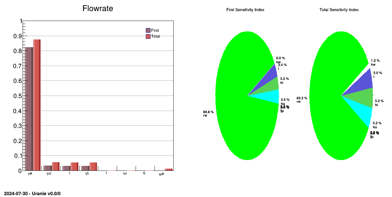
Processing sensitivitySobolLoadFile.py...

--- Uranie v4.11/0 --- Developed with ROOT (6.36.06)
                      Copyright (C) 2013-2026 CEA/DES
                      Contact: support-uranie@cea.fr
                      Date: Tue Feb 10, 2026

 <URANIE::WARNING>
 <URANIE::WARNING> *** URANIE WARNING ***
 <URANIE::WARNING> *** File[${SOURCEDIR}/dataSERVER/souRCE/TDataServer.cxx] Line[760]
 <URANIE::WARNING> TDataServer::fileDataRead: Expected iterator tdsflowreate_1__n__iter__ not found but tdsflowreate__n__iter__ looks like an URANIE iterator => Will be used as so.
 <URANIE::WARNING> *** END of URANIE WARNING ***
 <URANIE::WARNING>
 <URANIE::WARNING>
 <URANIE::WARNING> *** URANIE WARNING ***
 <URANIE::WARNING> *** File[${SOURCEDIR}/dataSERVER/souRCE/TDataServer.cxx] Line[8531]
 <URANIE::WARNING> TDataServer::getTuple Error : There is no tree!
 <URANIE::WARNING> *** END of URANIE WARNING ***
 <URANIE::WARNING>
 <URANIE::INFO>
 <URANIE::INFO> *** URANIE INFORMATION ***
 <URANIE::INFO> *** File[${SOURCEDIR}/meTIER/sampler/souRCE/TSamplerStochastic.cxx] Line[66]
 <URANIE::INFO> TSamplerStochastic::init: the TDS [tdsflowreate] contains data: we need to empty it !
 <URANIE::INFO> *** END of URANIE INFORMATION ***
 <URANIE::INFO>
 ** Case of Output atty [flowrateModel]  nSimPerIndex 20000
 ** Input att [rw] First [0.823516] Total Order[0.873849]
 ** Input att [r] First [0] Total Order[5.22438e-05]
 ** Input att [tu] First [0] Total Order[5e-05]
 ** Input att [tl] First [0] Total Order[6.08391e-05]
 ** Input att [hu] First [0.0319889] Total Order[0.0547724]
 ** Input att [hl] First [0.0304453] Total Order[0.0540884]
 ** Input att [l] First [0.0315935] Total Order[0.0527791]
 ** Input att [kw] First [0] Total Order[0.0129065]
************************************************************************************************************
*    Row   *   Out.Out *   Inp.Inp * Order.Ord * Method.Me * Algo.Algo * Value.Val * CILower.C * CIUpper.C *
************************************************************************************************************
*        0 * flowrateM *        rw *     First *     Sobol * --first-- * 0.8235162 * 0.8190045 * 0.8279262 *
*        4 * flowrateM *        rw *     Total *     Sobol * --total-- * 0.8738492 * 0.8602341 * 0.8875120 *
*        8 * flowrateM *         r *     First *     Sobol * --first-- *         0 *         0 * 0.0138594 *
*       12 * flowrateM *         r *     Total *     Sobol * --total-- * 5.224e-05 * 5.081e-05 * 5.371e-05 *
*       16 * flowrateM *        tu *     First *     Sobol * --first-- *         0 *         0 * 0.0138594 *
*       20 * flowrateM *        tu *     Total *     Sobol * --total-- * 5.000e-05 * 4.863e-05 * 5.140e-05 *
*       24 * flowrateM *        tl *     First *     Sobol * --first-- *         0 *         0 * 0.0138594 *
*       28 * flowrateM *        tl *     Total *     Sobol * --total-- * 6.083e-05 * 5.917e-05 * 6.254e-05 *
*       32 * flowrateM *        hu *     First *     Sobol * --first-- * 0.0319888 * 0.0181374 * 0.0458280 *
*       36 * flowrateM *        hu *     Total *     Sobol * --total-- * 0.0547723 * 0.0533147 * 0.0562686 *
*       40 * flowrateM *        hl *     First *     Sobol * --first-- * 0.0304453 * 0.0165929 * 0.0442861 *
*       44 * flowrateM *        hl *     Total *     Sobol * --total-- * 0.0540884 * 0.0526485 * 0.0555665 *
*       48 * flowrateM *         l *     First *     Sobol * --first-- * 0.0315935 * 0.0177418 * 0.0454330 *
*       52 * flowrateM *         l *     Total *     Sobol * --total-- * 0.0527791 * 0.0513732 * 0.0542224 *
*       56 * flowrateM *        kw *     First *     Sobol * --first-- *         0 *         0 * 0.0138594 *
*       60 * flowrateM *        kw *     Total *     Sobol * --total-- * 0.0129065 * 0.0125558 * 0.0132669 *
*       64 * flowrateM *   __sum__ *     First *     Sobol * --first-- * 0.9175440 *        -1 *        -1 *
*       65 * flowrateM *   __sum__ *     Total *     Sobol * --total-- * 1.0485587 *        -1 *        -1 *
************************************************************************************************************
==> 18 selected entries
The objective of this macro is to perform a sensitivity analysis using the Johnson's relative weight method on a
set of eight parameters used in the flowrateModel model described in Section IV.1.2.1.
"""
Example of Johnson relative weight method applied to flowrate
"""
from rootlogon import ROOT, DataServer, Sensitivity

ROOT.gROOT.LoadMacro("UserFunctions.C")

# Define the DataServer
tds = DataServer.TDataServer("tdsflowrate", "DataBase flowrate")
tds.addAttribute(DataServer.TUniformDistribution("rw", 0.05, 0.15))
tds.addAttribute(DataServer.TUniformDistribution("r", 100.0, 50000.0))
tds.addAttribute(DataServer.TUniformDistribution("tu", 63070.0, 115600.0))
tds.addAttribute(DataServer.TUniformDistribution("tl", 63.1, 116.0))
tds.addAttribute(DataServer.TUniformDistribution("hu", 990.0, 1110.0))
tds.addAttribute(DataServer.TUniformDistribution("hl", 700.0, 820.0))
tds.addAttribute(DataServer.TUniformDistribution("l", 1120.0, 1680.0))
tds.addAttribute(DataServer.TUniformDistribution("kw", 9855.0, 12045.0))

# param Size of a sampling.
nS = 1000
FuncName = "flowrateModel"

tjrw = Sensitivity.TJohnsonRW(tds, FuncName, nS,
                              "rw:r:tu:tl:hu:hl:l:kw", FuncName)
tjrw.computeIndexes()

# Get the results on screen
tjrw.getResultTuple().Scan("Out:Inp:Method:Value", "Order==\"First\"")

# Get the results as plots
cc = ROOT.TCanvas("canhist", "histgramme")
tjrw.drawIndexes("Flowrate", "", "nonewcanv,hist,first")
cc.Print("appliUranieFlowrateJohnsonRW1000Histogram_py.png")

ccc = ROOT.TCanvas("canpie", "TPie")
tjrw.drawIndexes("Flowrate", "", "nonewcanv,pie")
ccc.Print("appliUranieFlowrateJohnsonRW1000Pie_py.png")
The function flowrateModel is loaded from the macro UserFunctions.py
(the file can be found in ${URANIESYS}/share/uranie/macros)
ROOT.gROOT.LoadMacro("UserFunctions.C");
Each parameter is related to the TDataServer as a TAttribute and obeys an uniform law on specific
interval
## Define the DataServer
tds = DataServer.TDataServer("tdsflowrate", "DataBase flowrate");
tds.addAttribute( DataServer.TUniformDistribution("rw", 0.05, 0.15));
tds.addAttribute( DataServer.TUniformDistribution("r", 100.0, 50000.0));
tds.addAttribute( DataServer.TUniformDistribution("tu", 63070.0, 115600.0));
tds.addAttribute( DataServer.TUniformDistribution("tl", 63.1, 116.0));
tds.addAttribute( DataServer.TUniformDistribution("hu", 990.0, 1110.0));
tds.addAttribute( DataServer.TUniformDistribution("hl", 700.0, 820.0));
tds.addAttribute( DataServer.TUniformDistribution("l", 1120.0, 1680.0));
tds.addAttribute( DataServer.TUniformDistribution("kw", 9855.0, 12045.0));
To instantiate the TJohnsonRW object, one uses the TDataServer, the name of the function, the number
of samplings needed to perform sensitivity analysis (here =4000) and the input and output variables:
tjrw = Sensitivity.TJohnsonRW(tds, FuncName, nS, "rw:r:tu:tl:hu:hl:l:kw", FuncName);
Computation of sensitivity indexes:
trbd.computeIndexes();
The rest is very common to all sensitivity macros discussed here: it will produce two plots (the first one being a histogram show below) and the console is also shown below for completness.
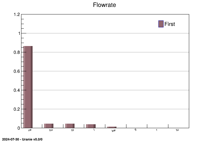
Processing sensitivityJohnsonRWFunctionFlowrate.py...

--- Uranie v4.11/0 --- Developed with ROOT (6.36.06)
                      Copyright (C) 2013-2026 CEA/DES
                      Contact: support-uranie@cea.fr
                      Date: Tue Feb 10, 2026

 <URANIE::WARNING>
 <URANIE::WARNING> *** URANIE WARNING ***
 <URANIE::WARNING> *** File[${SOURCEDIR}/dataSERVER/souRCE/TDataServer.cxx] Line[8531]
 <URANIE::WARNING> TDataServer::getTuple Error : There is no tree!
 <URANIE::WARNING> *** END of URANIE WARNING ***
 <URANIE::WARNING>
 <URANIE::INFO>
 <URANIE::INFO> *** URANIE INFORMATION ***
 <URANIE::INFO> *** File[${SOURCEDIR}/meTIER/sampler/souRCE/TSamplerStochastic.cxx] Line[66]
 <URANIE::INFO> TSamplerStochastic::init: the TDS [tdsflowrate] contains data: we need to empty it !
 <URANIE::INFO> *** END of URANIE INFORMATION ***
 <URANIE::INFO>
************************************************************
*    Row   *       Out *       Inp *    Method *     Value *
************************************************************
*        0 * flowrateM *        rw * JohnsonRW * 0.8636266 *
*        2 * flowrateM *         r * JohnsonRW * 4.598e-05 *
*        4 * flowrateM *        tu * JohnsonRW * 8.775e-06 *
*        6 * flowrateM *        tl * JohnsonRW * 9.689e-05 *
*        8 * flowrateM *        hu * JohnsonRW * 0.0439173 *
*       10 * flowrateM *        hl * JohnsonRW * 0.0435594 *
*       12 * flowrateM *         l * JohnsonRW * 0.0378304 *
*       14 * flowrateM *        kw * JohnsonRW * 0.0109144 *
*       16 * flowrateM *    __R2__ * JohnsonRW * 0.9447092 *
*       18 * flowrateM *   __R2A__ * JohnsonRW * 0.9442633 *
************************************************************
==> 10 selected entries
The objective of this macro is to perform a sensitivity analysis using the Johnson's relative weight method on a
set of eight parameters used in the flowrateModel model described in Section IV.1.2.1. Compared to version detailled in Section XIV.6.16, the idea is here to correlate the input variables
with a random correlation matrix.
"""
Example of Johson relative weight method applied to flowrate
"""
from math import sqrt
from rootlogon import ROOT, DataServer, Sensitivity


def gen_corr(_nx=8, correlated=True):
    """Generate randomly a good, highly-correlated, input correlation matrix."""

    # Define a randomly filled matrix
    a_mat = ROOT.TMatrixD(_nx, _nx)
    for i in range(_nx):
        for j in range(_nx):
            a_mat[i][j] = ROOT.gRandom.Gaus(0, 1)

    # Compute AA^T and normalise it to get "covariance matrix"
    gamma = ROOT.TMatrixD(a_mat, ROOT.TMatrixD.kMultTranspose, a_mat)
    gamma *= 1. / _nx

    # Inverse of the diagonal matrix to do as if this was 1/sqrt(variance)
    sig = ROOT.TMatrixD(_nx, _nx)
    for i in range(_nx):
        sig[i][i] = 1. / sqrt(gamma[i][i])

    # Compute the input correlation matrix
    in_corr_right = ROOT.TMatrixD(gamma, ROOT.TMatrixD.kMult, sig)
    in_corr = ROOT.TMatrixD(sig, ROOT.TMatrixD.kMult, in_corr_right)
    if not correlated:
        in_corr.UnitMatrix()

    return in_corr


ROOT.gROOT.LoadMacro("UserFunctions.C")

# Define the DataServer
tds = DataServer.TDataServer("tdsflowrate", "DataBase flowrate")
tds.addAttribute(DataServer.TUniformDistribution("rw", 0.05, 0.15))
tds.addAttribute(DataServer.TUniformDistribution("r", 100.0, 50000.0))
tds.addAttribute(DataServer.TUniformDistribution("tu", 63070.0, 115600.0))
tds.addAttribute(DataServer.TUniformDistribution("tl", 63.1, 116.0))
tds.addAttribute(DataServer.TUniformDistribution("hu", 990.0, 1110.0))
tds.addAttribute(DataServer.TUniformDistribution("hl", 700.0, 820.0))
tds.addAttribute(DataServer.TUniformDistribution("l", 1120.0, 1680.0))
tds.addAttribute(DataServer.TUniformDistribution("kw", 9855.0, 12045.0))

# \param Size of a sampling.
nS = 1000
FuncName = "flowrateModel"

# Get a correlation matrix for the inputs
inCorr = gen_corr(8, True)
inCorr.Print()

tjrw = Sensitivity.TJohnsonRW(tds, FuncName, nS,
                              "rw:r:tu:tl:hu:hl:l:kw", FuncName)
# Set the correlation
tjrw.setInputCorrelationMatrix(inCorr)
tjrw.computeIndexes()

# Get the results on screen
tjrw.getResultTuple().Scan("Out:Inp:Method:Value", "Order==\"First\"")

# Get the results as plots
cc = ROOT.TCanvas("canhist", "histgramme")
tjrw.drawIndexes("Flowrate", "", "nonewcanv, hist, first")
cc.Print("appliUranieFlowrateJohnsonRWCorrelated1000Histogram_py.png")

ccc = ROOT.TCanvas("canpie", "TPie")
tjrw.drawIndexes("Flowrate", "", "nonewcanv, pie")
ccc.Print("appliUranieFlowrateJohnsonRWCorrelated1000Pie_py.png")
The first function, called GenCorr, is not discussed, because it is really technical and
not really interesting here. The only thing to know is that it provides a proper correlation matrix: a
positive-definite symmetrical matrix.
The function flowrateModel is loaded from the macro UserFunctions.py
(the file can be found in ${URANIESYS}/share/uranie/macros)
ROOT.gROOT.LoadMacro("UserFunctions.C");
Compared to the discussion in Section XIV.6.16.2, the instantiation of the attributes and the
TJohnsonRW object is the same. The only difference is done when injecting the correlation
matrix, which is done in these lines:
## Get a correlation matrix for the inputs
inCorr=GenCorr(8,True);
tjrw = Sensitivity.TJohnsonRW(tds, FuncName, nS, "rw:r:tu:tl:hu:hl:l:kw", FuncName);
##Set the correlation
tjrw.setInputCorrelationMatrix(inCorr);
The computation of sensitivity indices can finally be done:
trbd.computeIndexes();The rest is very common to all sensitivity macros discussed here: it will produce two plots (the first one being a histogram show below) and the console is also shown below for completness.
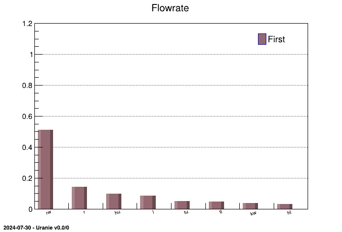
Processing sensitivityJohnsonRWCorrelatedFunctionFlowrate.py...

--- Uranie v4.11/0 --- Developed with ROOT (6.36.06)
                      Copyright (C) 2013-2026 CEA/DES
                      Contact: support-uranie@cea.fr
                      Date: Tue Feb 10, 2026


8x8 matrix is as follows

     |      0    |      1    |      2    |      3    |      4    |
----------------------------------------------------------------------
   0 |          1      0.4488      0.2894    -0.05727      0.3627
   1 |     0.4488           1     0.02022     -0.2547      0.3764
   2 |     0.2894     0.02022           1      0.4982     -0.2078
   3 |   -0.05727     -0.2547      0.4982           1     -0.9199
   4 |     0.3627      0.3764     -0.2078     -0.9199           1
   5 |     0.2569     -0.1996      -0.288      0.1004     -0.1362
   6 |    -0.2167     -0.4425    0.004268      0.1412      -0.111
   7 |    -0.2948      0.1982   -0.001661      0.1943     -0.3131


     |      5    |      6    |      7    |
----------------------------------------------------------------------
   0 |     0.2569     -0.2167     -0.2948
   1 |    -0.1996     -0.4425      0.1982
   2 |     -0.288    0.004268   -0.001661
   3 |     0.1004      0.1412      0.1943
   4 |    -0.1362      -0.111     -0.3131
   5 |          1     -0.1943      0.2848
   6 |    -0.1943           1     -0.4415
   7 |     0.2848     -0.4415           1

 <URANIE::WARNING>
 <URANIE::WARNING> *** URANIE WARNING ***
 <URANIE::WARNING> *** File[${SOURCEDIR}/dataSERVER/souRCE/TDataServer.cxx] Line[8531]
 <URANIE::WARNING> TDataServer::getTuple Error : There is no tree!
 <URANIE::WARNING> *** END of URANIE WARNING ***
 <URANIE::WARNING>
 <URANIE::INFO>
 <URANIE::INFO> *** URANIE INFORMATION ***
 <URANIE::INFO> *** File[${SOURCEDIR}/meTIER/sampler/souRCE/TSamplerStochastic.cxx] Line[66]
 <URANIE::INFO> TSamplerStochastic::init: the TDS [tdsflowrate] contains data: we need to empty it !
 <URANIE::INFO> *** END of URANIE INFORMATION ***
 <URANIE::INFO>
************************************************************
*    Row   *       Out *       Inp *    Method *     Value *
************************************************************
*        0 * flowrateM *        rw * JohnsonRW * 0.5113911 *
*        2 * flowrateM *         r * JohnsonRW * 0.1409327 *
*        4 * flowrateM *        tu * JohnsonRW * 0.0505176 *
*        6 * flowrateM *        tl * JohnsonRW * 0.0482684 *
*        8 * flowrateM *        hu * JohnsonRW * 0.0969452 *
*       10 * flowrateM *        hl * JohnsonRW * 0.0306674 *
*       12 * flowrateM *         l * JohnsonRW * 0.0836757 *
*       14 * flowrateM *        kw * JohnsonRW * 0.0376016 *
*       16 * flowrateM *    __R2__ * JohnsonRW * 0.9500813 *
*       18 * flowrateM *   __R2A__ * JohnsonRW * 0.9496787 *
************************************************************
==> 10 selected entries
The objective of this macro is to perform a sensitivity analysis using the Johnson's relative weight method on a
set of eight parameters which IS NOT the usual flowrateModel model. Indeed, compared to
version detailled in Section XIV.6.17,
the idea is here to correlate the input variables with a random correlation matrix and to translate this into a
full correlation matrix, meaning defining a "fake" output by computing their covariance with every input as if this
output was a perfect linear combination of these inputs.
An important particularity of this study is that no data are generated at all, it only uses the correlation matrix.
"""
Example of Johnson relative weight applied only to a correlation matrix
"""
from math import sqrt
from rootlogon import ROOT, DataServer, Sensitivity


def gen_corr(_nx=8, correlated=True):
    """Generate randomly a good, highly-correlated, correlation matrix for inputs
    define the proper covariance with the output to do as if this output if a
    perfect linear combination of the inputs."""

    # Define a randomly filled matrix
    a_mat = ROOT.TMatrixD(_nx, _nx)
    for i in range(_nx):
        for j in range(_nx):
            a_mat[i][j] = ROOT.gRandom.Gaus(0, 1)

    # Compute AA^T and normalise it to get "covariance matrix"
    gamma = ROOT.TMatrixD(a_mat, ROOT.TMatrixD.kMultTranspose, a_mat)
    gamma *= 1. / _nx

    # Inverse of the diagonal matrix to do as if this was 1/sqrt(variance)
    sig = ROOT.TMatrixD(_nx, _nx)
    for i in range(_nx):
        sig[i][i] = 1. / sqrt(gamma[i][i])

    # Compute the input correlation matrix
    in_corr_right = ROOT.TMatrixD(gamma, ROOT.TMatrixD.kMult, sig)
    in_corr = ROOT.TMatrixD(sig, ROOT.TMatrixD.kMult, in_corr_right)
    if not correlated:
        in_corr.UnitMatrix()
    var_y = in_corr.Sum()

    # Proper correlation, output included
    corr = ROOT.TMatrixD(_nx+1, _nx+1)
    corr.UnitMatrix()
    # putting already defined input
    corr.SetSub(0, 0, in_corr)
    # Adjust the covariance of the output wrt to all inputs
    for i in range(_nx):
        value = 0
        for j in range(_nx):
            value += in_corr[i][j]

        corr[_nx][i] = corr[i][_nx] = value / sqrt(var_y)

    return corr


# Define the DataServer
tds = DataServer.TDataServer("tdsflowrate", "DataBase flowrate")
tds.addAttribute("rw")
tds.addAttribute("r")
tds.addAttribute("tu")
tds.addAttribute("tl")
tds.addAttribute("hu")
tds.addAttribute("hl")
tds.addAttribute("l")
tds.addAttribute("kw")
# outputs
tds.addAttribute("flowrateModel")
tds.getAttribute("flowrateModel").setOutput()


# Get the full correlation matrix
inCorr = gen_corr(8, True)

# Johnson definition
tjrw = Sensitivity.TJohnsonRW(tds, "rw:r:tu:tl:hu:hl:l:kw", "flowrateModel")
# Putting the newly defined correlation that states our output
# as a perfect linear combination of inputs
tjrw.setCorrelationMatrix(inCorr)
tjrw.computeIndexes()

# Get the results on screen
tjrw.getResultTuple().Scan("Out:Inp:Method:Value", "Order==\"First\"")

# Get the results as plots
cc = ROOT.TCanvas("canhist", "histgramme")
tjrw.drawIndexes("Flowrate", "", "nonewcanv, hist, first")
cc.Print("appliUranieFakeFlowrateJohnsonRWCorrelationHistogram_py.png")

ccc = ROOT.TCanvas("canpie", "TPie")
tjrw.drawIndexes("Flowrate", "", "nonewcanv, pie")
ccc.Print("appliUranieFakeFlowrateJohnsonRWCorrelationPie_py.png")
The first function, called GenCorr, is not discussed, because it is really technical and
not really interesting here. The only thing to know is that it provides a proper correlation matrix: a
positive-definite symmetrical matrix for the input and it computes the covariance for a "fake" output that would be
a perfect linear combination of all the inputs.
Because of this, the function flowrateModel is not loaded anymore and the definition of
the attributes is not the same: it is not necessary to use TStochasticAttribute because no
data are generated here:
## Define the DataServer
tds = DataServer.TDataServer("tdsflowrate", "DataBase flowrate");
tds.addAttribute("rw");
tds.addAttribute("r");
tds.addAttribute("tu");
tds.addAttribute("tl");
tds.addAttribute("hu");
tds.addAttribute("hl");
tds.addAttribute("l");
tds.addAttribute("kw");
## outputs
tds.addAttribute("flowrateModel");
tds.getAttribute("flowrateModel").setOutput();
Compared to the discussion in Section XIV.6.17.2, the only differences are the
instantiation of the TJohnsonRW object and the method code to provide the correlation
matrix.
## Get the full correlation matrix
inCorr=GenCorr(8,True);
## Johnson definition
tjrw = Sensitivity.TJohnsonRW(tds, "rw:r:tu:tl:hu:hl:l:kw", "flowrateModel");
##Putting the newly defined correlation that states our output as a perfect linear combination of inputs
tjrw.setCorrelationMatrix(inCorr);
The method called to provide the correlation matrix is setCorrelationMatrix and it means
that the user give a full correlation matrix (input and output variables), on the contrary to the one used in Section XIV.6.17.2 which is
setInputCorrelationMatrix, which set only the input correlation matrix.
The computation of sensitivity indices can finally be done:
trbd.computeIndexes();The rest is very common to all sensitivity macros discussed here: it will produce two plots (the first one being a histogram show below) and the console is also shown below for completness.
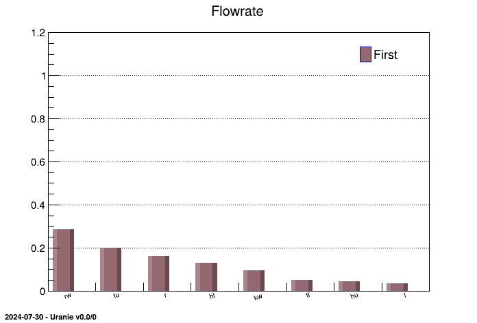
Processing sensitivityJohnsonRWJustCorrelationFakeFlowrate.py...

--- Uranie v4.11/0 --- Developed with ROOT (6.36.06)
                      Copyright (C) 2013-2026 CEA/DES
                      Contact: support-uranie@cea.fr
                      Date: Tue Feb 10, 2026

 <URANIE::WARNING>
 <URANIE::WARNING> *** URANIE WARNING ***
 <URANIE::WARNING> *** File[${SOURCEDIR}/dataSERVER/souRCE/TDataServer.cxx] Line[2202]
 <URANIE::WARNING> TDataServer::getNPatterns[tdsflowrate] WARNING
 <URANIE::WARNING>  The TTree is NULL
 <URANIE::WARNING> *** END of URANIE WARNING ***
 <URANIE::WARNING>
 <URANIE::WARNING>
 <URANIE::WARNING> *** URANIE WARNING ***
 <URANIE::WARNING> *** File[${SOURCEDIR}/meTIER/sensitivity/souRCE/TSensitivity.cxx] Line[165]
 <URANIE::WARNING> TSensitivity::constructor   ERROR The TTree is empty []
 <URANIE::WARNING> *** END of URANIE WARNING ***
 <URANIE::WARNING>
 <URANIE::WARNING>
 <URANIE::WARNING> *** URANIE WARNING ***
 <URANIE::WARNING> *** File[${SOURCEDIR}/dataSERVER/souRCE/TDataServer.cxx] Line[8531]
 <URANIE::WARNING> TDataServer::getTuple Error : There is no tree!
 <URANIE::WARNING> *** END of URANIE WARNING ***
 <URANIE::WARNING>
************************************************************
*    Row   *       Out *       Inp *    Method *     Value *
************************************************************
*        0 * flowrateM *        rw * JohnsonRW * 0.2844573 *
*        2 * flowrateM *         r * JohnsonRW * 0.1600467 *
*        4 * flowrateM *        tu * JohnsonRW * 0.2004196 *
*        6 * flowrateM *        tl * JohnsonRW * 0.0512434 *
*        8 * flowrateM *        hu * JohnsonRW * 0.0446220 *
*       10 * flowrateM *        hl * JohnsonRW * 0.1295644 *
*       12 * flowrateM *         l * JohnsonRW * 0.0333889 *
*       14 * flowrateM *        kw * JohnsonRW * 0.0962574 *
*       16 * flowrateM *    __R2__ * JohnsonRW *         1 *
************************************************************
==> 9 selected entries
The objective of this macro is to perform a sensitivity analysis using the HSIC method on a
set of eight parameters used in the flowrateModel model described in Section IV.1.2.1.
"""
Example of HSIC method applied to flowrate
"""
from rootlogon import ROOT, DataServer, Sensitivity, Launcher, Sampler
ROOT.gROOT.LoadMacro("UserFunctions.C")

# Define the DataServer
tds = DataServer.TDataServer("tdsflowrate", "DataBase flowrate")
tds.addAttribute(DataServer.TUniformDistribution("rw", 0.05, 0.15))
tds.addAttribute(DataServer.TUniformDistribution("r", 100.0, 50000.0))
tds.addAttribute(DataServer.TUniformDistribution("tu", 63070.0, 115600.0))
tds.addAttribute(DataServer.TUniformDistribution("tl", 63.1, 116.0))
tds.addAttribute(DataServer.TUniformDistribution("hu", 990.0, 1110.0))
tds.addAttribute(DataServer.TUniformDistribution("hl", 700.0, 820.0))
tds.addAttribute(DataServer.TUniformDistribution("l", 1120.0, 1680.0))
tds.addAttribute(DataServer.TUniformDistribution("kw", 9855.0, 12045.0))

# Generation of the sample (it can be a given sample).
nS = 500
sampling = Sampler.TSampling(tds, "lhs", nS);

sampling.generateSample();

tlf = Launcher.TLauncherFunction(tds, "flowrateModel");
tlf.setDrawProgressBar(False);
tlf.run();

# Create a THSIC object, compute indexes and print results
thsic = Sensitivity.THSIC(tds, "rw:r:tu:tl:hu:hl:l:kw","flowrateModel");
thsic.computeIndexes("quiet")
thsic.getResultTuple().SetScanField(60);
thsic.getResultTuple().Scan("Out:Inp:Method:Order:Value:CILower:CIUpper");

# Print HSIC indexes
can = ROOT.TCanvas("c1", "Graph sensitivityHSICFunctionFlowrate", 5, 64, 1270, 667)
thsic.drawIndexes("Flowrate", "", "hist, first, nonewcanv")
The function flowrateModel is loaded from the macro UserFunctions.C
(the file can be found in ${URANIESYS}/share/uranie/macros)
ROOT.gROOT.LoadMacro("UserFunctions.C");
Each parameter is related to the TDataServer as a TAttribute and obeys an uniform law on specific
interval
## Define the DataServer
tds = DataServer.TDataServer("tdsflowrate", "DataBase flowrate");
tds.addAttribute( DataServer.TUniformDistribution("rw", 0.05, 0.15));
tds.addAttribute( DataServer.TUniformDistribution("r", 100.0, 50000.0));
tds.addAttribute( DataServer.TUniformDistribution("tu", 63070.0, 115600.0));
tds.addAttribute( DataServer.TUniformDistribution("tl", 63.1, 116.0));
tds.addAttribute( DataServer.TUniformDistribution("hu", 990.0, 1110.0));
tds.addAttribute( DataServer.TUniformDistribution("hl", 700.0, 820.0));
tds.addAttribute( DataServer.TUniformDistribution("l", 1120.0, 1680.0));
tds.addAttribute( DataServer.TUniformDistribution("kw", 9855.0, 12045.0));
HSIC does not need a specific DOE, it works with a given sample. We generate a sample with TSampling and we evaluate it using TLauncherFunction
nS = 500
sampling = Sampler.TSampling(tds, "lhs", nS)
sampling.generateSample()
ROOT.gROOT.LoadMacro("UserFunctions.C")
tlf.setDrawProgressBar(False);
tlf.run();
To instantiate the THSIC object, one uses the TDataServer, the name of the input and output variables:
thsic = Sensitivity.THSIC(tds, "rw:r:tu:tl:hu:hl:l:kw", "flowaretModel");
Computation of sensitivity indexes:
thsic.computeIndexes();
It will produce one plots containing the HSIC indexes and the p-value to test the Independance between inputs and outputs.The console is also shown below for completness.
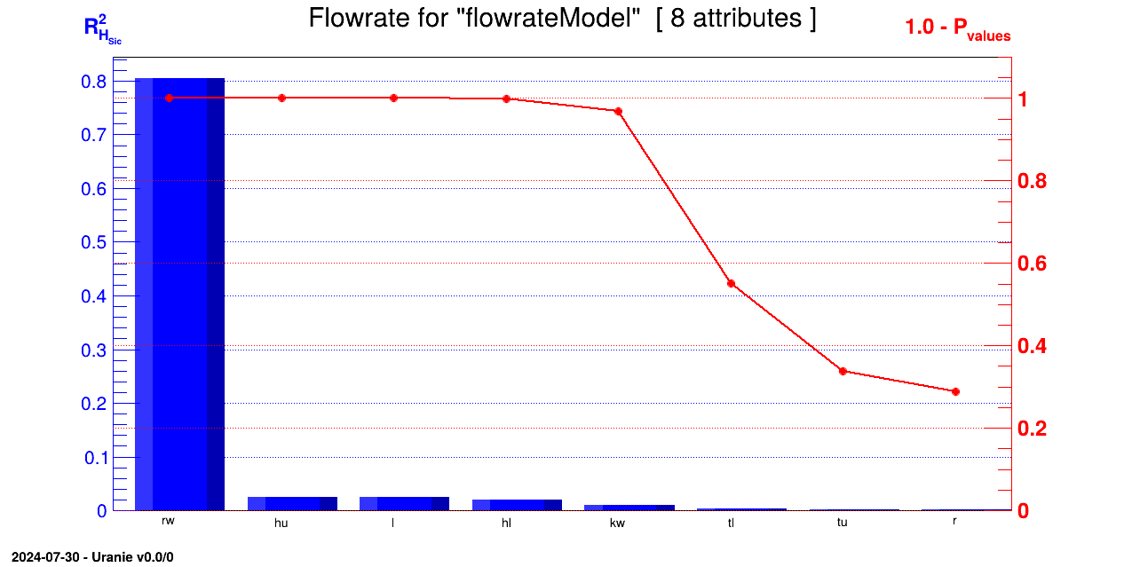
Processing sensitivityHSICFunctionFlowrate.py...

--- Uranie v4.11/0 --- Developed with ROOT (6.36.06)
                      Copyright (C) 2013-2026 CEA/DES
                      Contact: support-uranie@cea.fr
                      Date: Tue Feb 10, 2026

*************************************************************************************
*    Row   *    Out *      Inp * Metho *     Order *    Value *  CILower *  CIUpper *
*************************************************************************************
*        0 * flowra *       rw *  HSic *    R2HSic * 0.804431 *       -1 *       -1 *
*        1 * flowra *       rw *  HSic *      HSic * 0.072723 *       -1 *       -1 *
*        2 * flowra *       rw *  HSic *   pValues * 6.8e-106 *       -1 *       -1 *
*        3 * flowra *        r *  HSic *    R2HSic * 0.002238 *       -1 *       -1 *
*        4 * flowra *        r *  HSic *      HSic * 0.000202 *       -1 *       -1 *
*        5 * flowra *        r *  HSic *   pValues * 0.712174 *       -1 *       -1 *
*        6 * flowra *       tu *  HSic *    R2HSic * 0.002528 *       -1 *       -1 *
*        7 * flowra *       tu *  HSic *      HSic * 0.000228 *       -1 *       -1 *
*        8 * flowra *       tu *  HSic *   pValues * 0.662668 *       -1 *       -1 *
*        9 * flowra *       tl *  HSic *    R2HSic * 0.003806 *       -1 *       -1 *
*       10 * flowra *       tl *  HSic *      HSic * 0.000344 *       -1 *       -1 *
*       11 * flowra *       tl *  HSic *   pValues * 0.449068 *       -1 *       -1 *
*       12 * flowra *       hu *  HSic *    R2HSic * 0.025554 *       -1 *       -1 *
*       13 * flowra *       hu *  HSic *      HSic * 0.002309 *       -1 *       -1 *
*       14 * flowra *       hu *  HSic *   pValues * 3.13e-05 *       -1 *       -1 *
*       15 * flowra *       hl *  HSic *    R2HSic * 0.020243 *       -1 *       -1 *
*       16 * flowra *       hl *  HSic *      HSic * 0.001829 *       -1 *       -1 *
*       17 * flowra *       hl *  HSic *   pValues * 0.000445 *       -1 *       -1 *
*       18 * flowra *        l *  HSic *    R2HSic * 0.024934 *       -1 *       -1 *
*       19 * flowra *        l *  HSic *      HSic * 0.002253 *       -1 *       -1 *
*       20 * flowra *        l *  HSic *   pValues * 5.64e-05 *       -1 *       -1 *
*       21 * flowra *       kw *  HSic *    R2HSic * 0.010567 *       -1 *       -1 *
*       22 * flowra *       kw *  HSic *      HSic * 0.000955 *       -1 *       -1 *
*       23 * flowra *       kw *  HSic *   pValues * 0.032459 *       -1 *       -1 *
*************************************************************************************
The objective of this macro is to perform a sensitivity analysis using the SobolRank method on a
set of eight parameters used in the flowrateModel model described in Section IV.1.2.1.
"""
Example of HSIC method applied to flowrate
"""
from rootlogon import ROOT, DataServer, Sensitivity, Launcher, Sampler
ROOT.gROOT.LoadMacro("UserFunctions.C")

# Define the DataServer
tds = DataServer.TDataServer("tdsflowrate", "DataBase flowrate")
tds.addAttribute(DataServer.TUniformDistribution("rw", 0.05, 0.15))
tds.addAttribute(DataServer.TUniformDistribution("r", 100.0, 50000.0))
tds.addAttribute(DataServer.TUniformDistribution("tu", 63070.0, 115600.0))
tds.addAttribute(DataServer.TUniformDistribution("tl", 63.1, 116.0))
tds.addAttribute(DataServer.TUniformDistribution("hu", 990.0, 1110.0))
tds.addAttribute(DataServer.TUniformDistribution("hl", 700.0, 820.0))
tds.addAttribute(DataServer.TUniformDistribution("l", 1120.0, 1680.0))
tds.addAttribute(DataServer.TUniformDistribution("kw", 9855.0, 12045.0))

# Generation of the sample (it can be a given sample).
nS = 500
sampling = Sampler.TSampling(tds, "lhs", nS);

sampling.generateSample();

tlf = Launcher.TLauncherFunction(tds, "flowrateModel");
tlf.setDrawProgressBar(False);
tlf.run();

# Create a TSobolRank object, compute indexes and print results
tsobolrank = Sensitivity.TSobolRank(tds, "rw:r:tu:tl:hu:hl:l:kw","flowrateModel");
tsobolrank.computeIndexes()
tsobolrank.getResultTuple().SetScanField(60);
tsobolrank.getResultTuple().Scan("Out:Inp:Method:Order:Value:CILower:CIUpper");

# Print Sobol indexes
can = ROOT.TCanvas("c1", "Graph sensitivitySobolRankFunctionFlowrate", 5, 64, 1270, 667)
tsobolrank.drawIndexes("Flowrate", "", "hist, first, nonewcanv")
The function flowrateModel is loaded from the macro UserFunctions.C
(the file can be found in ${URANIESYS}/share/uranie/macros)
ROOT.gROOT.LoadMacro("UserFunctions.C");
Each parameter is related to the TDataServer as a TAttribute and obeys an uniform law on specific
interval
## Define the DataServer
tds = DataServer.TDataServer("tdsflowrate", "DataBase flowrate");
tds.addAttribute( DataServer.TUniformDistribution("rw", 0.05, 0.15));
tds.addAttribute( DataServer.TUniformDistribution("r", 100.0, 50000.0));
tds.addAttribute( DataServer.TUniformDistribution("tu", 63070.0, 115600.0));
tds.addAttribute( DataServer.TUniformDistribution("tl", 63.1, 116.0));
tds.addAttribute( DataServer.TUniformDistribution("hu", 990.0, 1110.0));
tds.addAttribute( DataServer.TUniformDistribution("hl", 700.0, 820.0));
tds.addAttribute( DataServer.TUniformDistribution("l", 1120.0, 1680.0));
tds.addAttribute( DataServer.TUniformDistribution("kw", 9855.0, 12045.0));
HSIC does not need a specific DOE, it works with a given sample. We generate a sample with TSampling and we evaluate it using TLauncherFunction
nS = 500
sampling = Sampler.TSampling(tds, "lhs", nS)
sampling.generateSample()
ROOT.gROOT.LoadMacro("UserFunctions.C")
tlf.setDrawProgressBar(False);
tlf.run();
To instantiate the TSobolRank object, one uses the TDataServer, the name of the input and output variables:
tsobolrank = Sensitivity.TSobolRank(tds, "rw:r:tu:tl:hu:hl:l:kw", "flowaretModel");
Computation of sensitivity indexes:
tsobolrank.computeIndexes();
It will produce one plots containing the SobolRank indexes and the p-value to test the Independance between inputs and outputs.The console is also shown below for completness.
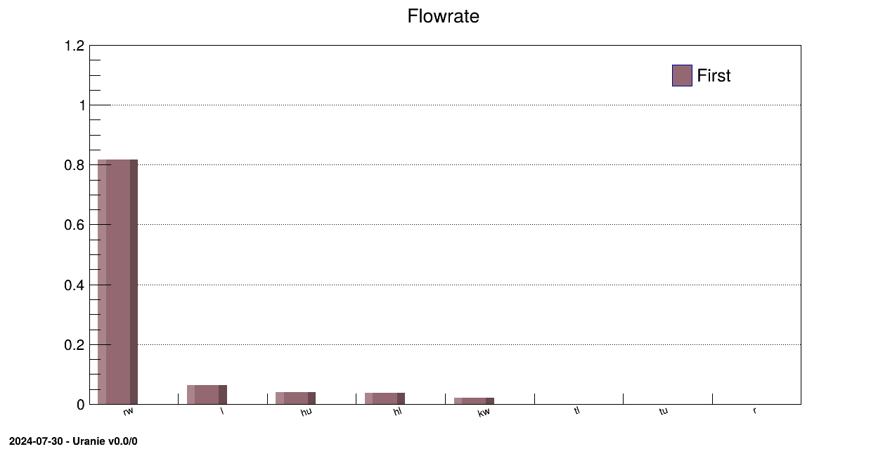
Processing sensitivitySobolRankFunctionFlowrate.py...

--- Uranie v4.11/0 --- Developed with ROOT (6.36.06)
                      Copyright (C) 2013-2026 CEA/DES
                      Contact: support-uranie@cea.fr
                      Date: Tue Feb 10, 2026

*************************************************************************************
*    Row   *    Out *      Inp * Metho *     Order *    Value *  CILower *  CIUpper *
*************************************************************************************
*        0 * flowra *       rw * Sobol *     First * 0.816872 *       -1 *       -1 *
*        1 * flowra *        r * Sobol *     First * -0.04759 *       -1 *       -1 *
*        2 * flowra *       tu * Sobol *     First * -0.04164 *       -1 *       -1 *
*        3 * flowra *       tl * Sobol *     First * -0.00414 *       -1 *       -1 *
*        4 * flowra *       hu * Sobol *     First * 0.041272 *       -1 *       -1 *
*        5 * flowra *       hl * Sobol *     First * 0.036748 *       -1 *       -1 *
*        6 * flowra *        l * Sobol *     First * 0.062867 *       -1 *       -1 *
*        7 * flowra *       kw * Sobol *     First * 0.021273 *       -1 *       -1 *
*************************************************************************************
The objective of this macro is to perform a sensitivity analysis using the Cramer Von Mises method on a
set of eight parameters used in the flowrateModel model described in Section IV.1.2.1.
"""
Example of Cramer Von Mises estimation for the flowrate function
"""
import ROOT
from ROOT.URANIE import DataServer, Sensitivity

from rootlogon import ROOT, DataServer, Sensitivity

ROOT.gROOT.LoadMacro("UserFunctions.C")

# Define the DataServer
tds = DataServer.TDataServer("tdsflowreate", "DataBase flowreate")
tds.addAttribute(DataServer.TUniformDistribution("rw", 0.05, 0.15))
tds.addAttribute(DataServer.TUniformDistribution("r", 100.0, 50000.0))
tds.addAttribute(DataServer.TUniformDistribution("tu", 63070.0, 115600.0))
tds.addAttribute(DataServer.TUniformDistribution("tl", 63.1, 116.0))
tds.addAttribute(DataServer.TUniformDistribution("hu", 990.0, 1110.0))
tds.addAttribute(DataServer.TUniformDistribution("hl", 700.0, 820.0))
tds.addAttribute(DataServer.TUniformDistribution("l", 1120.0, 1680.0))
tds.addAttribute(DataServer.TUniformDistribution("kw", 9855.0, 12045.0))

ns = 10000
tcvm = Sensitivity.TCramerVonMises(tds, "flowrateModel", ns, "rw:r:tu:tl:hu:hl:l:kw",
                            "flowrateModel", "DummyPython")
tcvm.setDrawProgressBar(False)
tcvm.computeIndexes()

tcvm.getResultTuple().Scan("*", "Method==\"CramerVonMises\"")

cc = ROOT.TCanvas("c1", "histgramme", 5, 64, 1270, 667)
pad = ROOT.TPad("pad", "pad", 0, 0.03, 1, 1)
pad.Draw()
pad.Divide(2, 1)
pad.cd(1)
tcvm.drawIndexes("Flowrate", "", "nonewcanv, hist, all")

pad.cd(2)
tcvm.drawIndexes("Flowrate", "", "nonewcanv, pie, first")
The function flowrateModel is loaded from the macro UserFunctions.C
(the file can be found in ${URANIESYS}/share/uranie/macros)
ROOT.gROOT.LoadMacro("UserFunctions.C");
Each parameter is related to the TDataServer as a TAttribute and obeys an uniform law on specific
interval
# Define the DataServer
tds = DataServer.TDataServer("tdsflowreate", "DataBase flowreate")
tds.addAttribute(DataServer.TUniformDistribution("rw", 0.05, 0.15))
tds.addAttribute(DataServer.TUniformDistribution("r", 100.0, 50000.0))
tds.addAttribute(DataServer.TUniformDistribution("tu", 63070.0, 115600.0))
tds.addAttribute(DataServer.TUniformDistribution("tl", 63.1, 116.0))
tds.addAttribute(DataServer.TUniformDistribution("hu", 990.0, 1110.0))
tds.addAttribute(DataServer.TUniformDistribution("hl", 700.0, 820.0))
tds.addAttribute(DataServer.TUniformDistribution("l", 1120.0, 1680.0))
tds.addAttribute(DataServer.TUniformDistribution("kw", 9855.0, 12045.0))
CramerVonMises is a extension of the pick and freeze DOE use for Sobol method.
To instantiate the TCramerVonMises object, one uses the TDataServer, the name of the function and the number of samplings
needed to perform sensitivity analysis (here ns=10000):
tcvm = Sensitivity.TCramerVonMises(tds, "flowrateModel", ns, "rw:r:tu:tl:hu:hl:l:kw", "flowrateModel");
Computation of sensitivity indexes:
tcvm.computeIndexes();
As CramerVonMises is a extension of the pick and freeze DOE use for Sobol method, the Sobol indices are also computed.
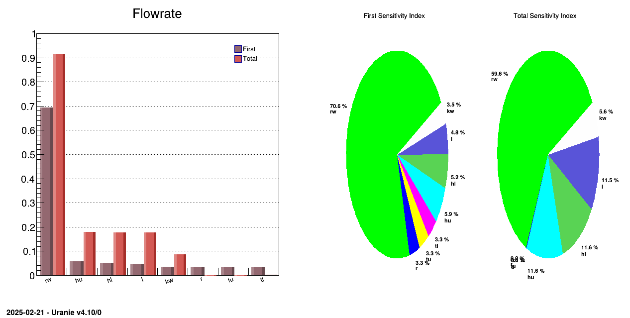
Processing sensitivityCramerVonMisesFunctionFlowrate.py...

--- Uranie v4.11/0 --- Developed with ROOT (6.36.06)
                      Copyright (C) 2013-2026 CEA/DES
                      Contact: support-uranie@cea.fr
                      Date: Tue Feb 10, 2026

 <URANIE::WARNING>
 <URANIE::WARNING> *** URANIE WARNING ***
 <URANIE::WARNING> *** File[${SOURCEDIR}/dataSERVER/souRCE/TDataServer.cxx] Line[8531]
 <URANIE::WARNING> TDataServer::getTuple Error : There is no tree!
 <URANIE::WARNING> *** END of URANIE WARNING ***
 <URANIE::WARNING>
 <URANIE::INFO>
 <URANIE::INFO> *** URANIE INFORMATION ***
 <URANIE::INFO> *** File[${SOURCEDIR}/meTIER/sampler/souRCE/TSamplerStochastic.cxx] Line[66]
 <URANIE::INFO> TSamplerStochastic::init: the TDS [tdsflowreate] contains data: we need to empty it !
 <URANIE::INFO> *** END of URANIE INFORMATION ***
 <URANIE::INFO>
 ** Case of Output atty [flowrateModel]  nSimPerIndex 910
 ** Input att [rw] First CVM [0.694231] Total Order CVM[0.913107]
 ** Input att [r] First CVM [0.0327274] Total Order CVM[0.000562551]
 ** Input att [tu] First CVM [0.0326926] Total Order CVM[0]
 ** Input att [tl] First CVM [0.0326247] Total Order CVM[0.00153446]
 ** Input att [hu] First CVM [0.0582536] Total Order CVM[0.17845]
 ** Input att [hl] First CVM [0.0515417] Total Order CVM[0.177485]
 ** Input att [l] First CVM [0.0469543] Total Order CVM[0.176094]
 ** Input att [kw] First CVM [0.0343777] Total Order CVM[0.0857252]
************************************************************************************************************
*    Row   *   Out.Out *   Inp.Inp * Order.Ord * Method.Me * Algo.Algo * Value.Val * CILower.C * CIUpper.C *
************************************************************************************************************
*       66 * flowrateM *        rw *  FirstCVM * CramerVon * --first-- * 0.6942309 *        -1 *        -1 *
*       67 * flowrateM *        rw *  TotalCVM * CramerVon * --total-- * 0.9131074 *        -1 *        -1 *
*       68 * flowrateM *         r *  FirstCVM * CramerVon * --first-- * 0.0327273 *        -1 *        -1 *
*       69 * flowrateM *         r *  TotalCVM * CramerVon * --total-- * 0.0005625 *        -1 *        -1 *
*       70 * flowrateM *        tu *  FirstCVM * CramerVon * --first-- * 0.0326926 *        -1 *        -1 *
*       71 * flowrateM *        tu *  TotalCVM * CramerVon * --total-- *         0 *        -1 *        -1 *
*       72 * flowrateM *        tl *  FirstCVM * CramerVon * --first-- * 0.0326246 *        -1 *        -1 *
*       73 * flowrateM *        tl *  TotalCVM * CramerVon * --total-- * 0.0015344 *        -1 *        -1 *
*       74 * flowrateM *        hu *  FirstCVM * CramerVon * --first-- * 0.0582536 *        -1 *        -1 *
*       75 * flowrateM *        hu *  TotalCVM * CramerVon * --total-- * 0.1784495 *        -1 *        -1 *
*       76 * flowrateM *        hl *  FirstCVM * CramerVon * --first-- * 0.0515417 *        -1 *        -1 *
*       77 * flowrateM *        hl *  TotalCVM * CramerVon * --total-- * 0.1774852 *        -1 *        -1 *
*       78 * flowrateM *         l *  FirstCVM * CramerVon * --first-- * 0.0469543 *        -1 *        -1 *
*       79 * flowrateM *         l *  TotalCVM * CramerVon * --total-- * 0.1760940 *        -1 *        -1 *
*       80 * flowrateM *        kw *  FirstCVM * CramerVon * --first-- * 0.0343777 *        -1 *        -1 *
*       81 * flowrateM *        kw *  TotalCVM * CramerVon * --total-- * 0.0857252 *        -1 *        -1 *
*       82 * flowrateM *   __sum__ *  FirstCVM * CramerVon * --first-- * 0.9834030 *        -1 *        -1 *
*       83 * flowrateM *   __sum__ *  TotalCVM * CramerVon * --total-- * 1.5329584 *        -1 *        -1 *
************************************************************************************************************
==> 18 selected entries
| |  | |
| XIV.5. Macros Launcher |  | XIV.7. Macros Modeler |