Documentation / Manuel utilisateur en Python :

The objective of the macro is to build a multilinear regression between the predictors related to the normalisation of the variables x1, x2, x3, x4, x5, x6, x7 and a target variable y from the database contained in the ASCII file cornell.dat:

#NAME: cornell
#TITLE: Dataset Cornell 1990
#COLUMN_NAMES: x1 | x2 | x3 | x4 | x5 | x6 | x7 | y
#COLUMN_TITLES: x_{1} | x_{2} | x_{3} | x_{4} | x_{5} | x_{6} | x_{7} | y

0.00 0.23 0.00 0.00 0.00 0.74 0.03 98.7
0.00 0.10 0.00 0.00 0.12 0.74 0.04 97.8
0.00 0.00 0.00 0.10 0.12 0.74 0.04 96.6
0.00 0.49 0.00 0.00 0.12 0.37 0.02 92.0
0.00 0.00 0.00 0.62 0.12 0.18 0.08 86.6
0.00 0.62 0.00 0.00 0.00 0.37 0.01 91.2
0.17 0.27 0.10 0.38 0.00 0.00 0.08 81.9
0.17 0.19 0.10 0.38 0.02 0.06 0.08 83.1
0.17 0.21 0.10 0.38 0.00 0.06 0.08 82.4
0.17 0.15 0.10 0.38 0.02 0.10 0.08 83.2
0.21 0.36 0.12 0.25 0.00 0.00 0.06 81.4
0.00 0.00 0.00 0.55 0.00 0.37 0.08 88.1

"""
Example of linear regression model
"""
from rootlogon import ROOT, DataServer, Modeler

tds = DataServer.TDataServer()
tds.fileDataRead("cornell.dat")

tds.normalize("*", "cr")  # "*" is equivalent to "x1:x2:x3:x4:x5:x6:y"
# Third field not filled implies DataServer.TDataServer.kCR

c = ROOT.TCanvas("c1", "Graph for the Macro modeler", 5, 64, 1270, 667)
pad = ROOT.TPad("pad", "pad", 0, 0.03, 1, 1)
pad.Draw()
pad.Divide(2)
pad.cd(1)
tds.draw("y:x7")

tlin = Modeler.TLinearRegression(tds, "x1cr:x2cr:x3cr:x4cr:x5cr:x6cr",
                                 "ycr", "nointercept")
tlin.estimate()

pad.cd(2)
tds.draw("ycr:ycrhat")

The ASCII data file cornell.dat is loaded in the TDataServer:

tds = DataServer.TDataServer();
tds.fileDataRead("cornell.dat");

The variables are all normalised with a standardised method. The normalised attributes are created with the cr extension:

tds.normalize("*", "cr");

The linear regression is initialised and characteristic values are computed for each normalised variable with the estimate method. The regression is built with no intercept:

tlin=Modeler.TLinearRegression(tds,"x1cr:x2cr:x3cr:x4cr:x5cr:x6cr", "ycr", "nointercept");
tlin.estimate();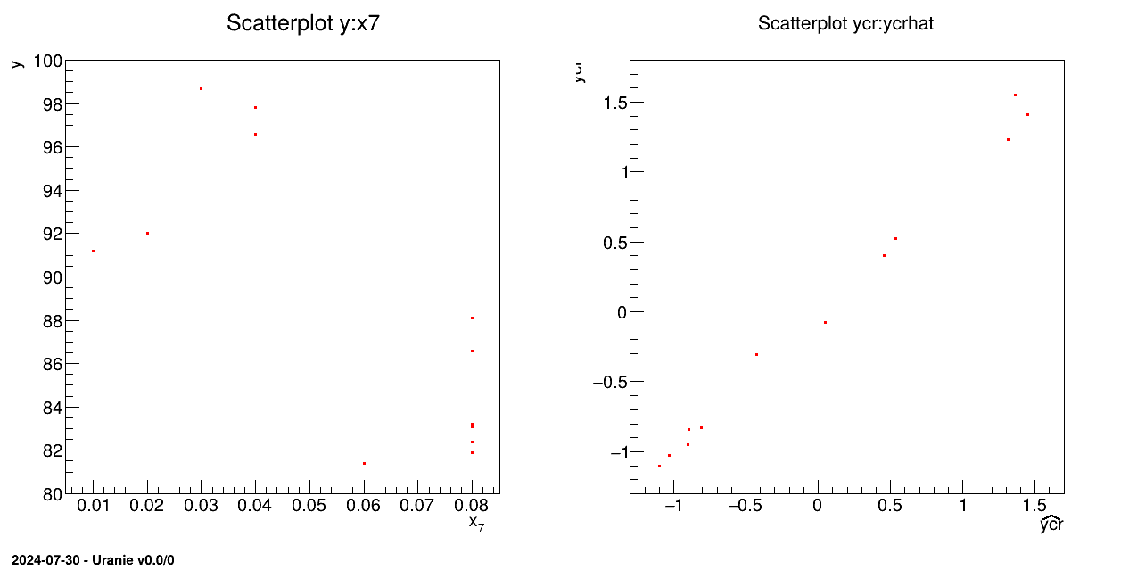

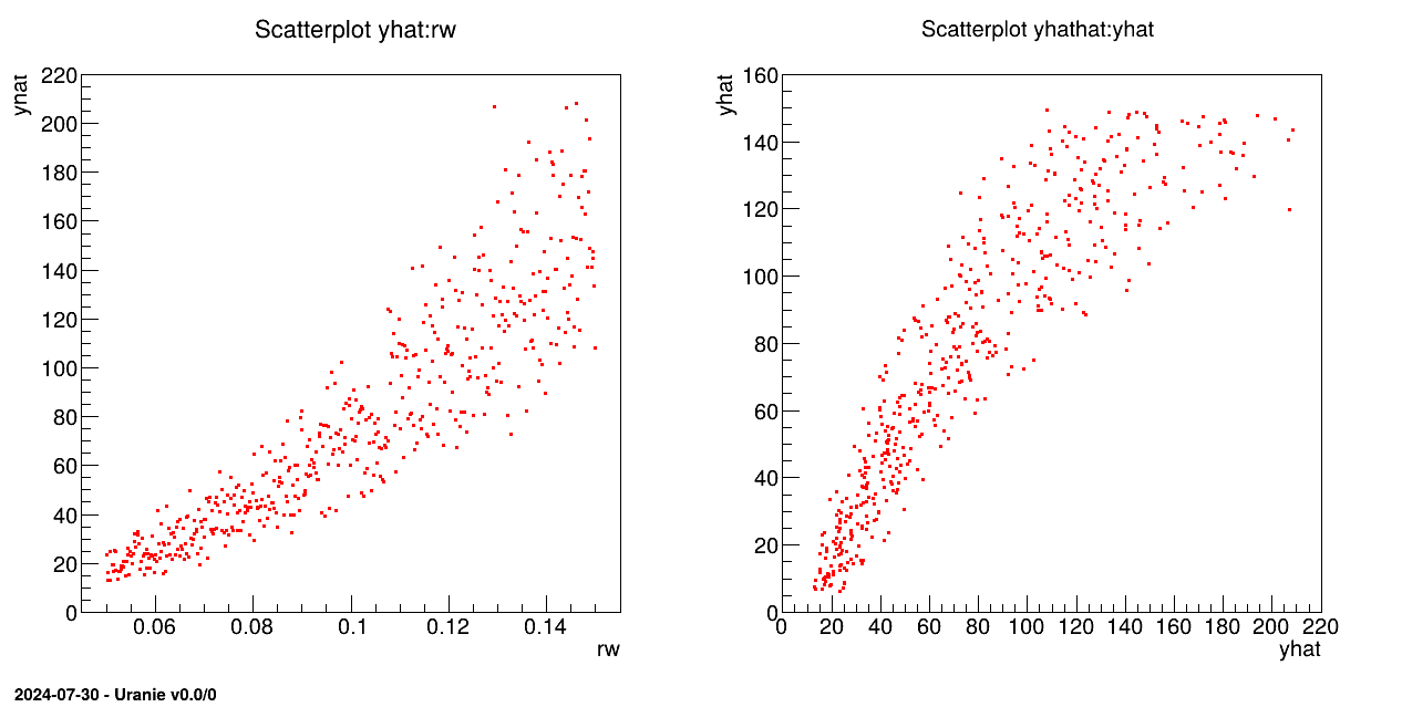
The objective of this macro is to build a linear regression between a predictor rw and a target variable yhat from the database contained in the ASCII file flowrate_sampler_launcher_500.dat defining values for the eight variables described in Section IV.1.2.1 on 500 patterns.

"""
Example of linear regression on flowrate
"""
from rootlogon import ROOT, DataServer, Modeler

tds = DataServer.TDataServer()
tds.fileDataRead("flowrate_sampler_launcher_500.dat")

c = ROOT.TCanvas("c1", "Graph for the Macro modeler", 5, 64, 1270, 667)
pad = ROOT.TPad("pad", "pad", 0, 0.03, 1, 1)
pad.Draw()
pad.Divide(2)
pad.cd(1)
tds.draw("yhat:rw")

# tds.getAttribute("yhat").setOutput()

tlin = Modeler.TLinearRegression(tds, "rw", "yhat", "DummyForPython")
tlin.estimate()

pad.cd(2)
tds.draw("yhathat:yhat")

tds.startViewer()

The TDataServer is loaded with the database contained in the file flowrate_sampler_launcher_500.dat with the fileDataRead method:

tds=DataServer.TDataServer();
tds.fileDataRead("flowrate_sampler_launcher_500.dat");

The linear regression is initialised and characteristic values are computed for rw with the estimate method:

tlin=Modeler.TLinearRegression(tds, "rw","yhat", "DummyForPython");
tlin.estimate();

The last argument is the option field, which in most cases is empty. Here it is filled with "DummyPython" which helps specify to python which constructor to choose. There are indeed several possible constructors these 5 five first arguments, but C++ can make the difference between them as the literal members are either std::string, ROOT::TString, Char_t* or even Option_t*. For python, these format are all PyString, so the sixth argument is compulsory to disentangle the possibilities.

The objective of the macro is to build a multilinear regression between the predictors , , , , , , , and a target variable yhat from the database contained in the ASCII file flowrate_sampler_launcher_500.dat defining values for these eight variables described in Section IV.1.2.1 on 500 patterns. Parameters of the regression are then exported in a .py file _FileContainingFunction_.C:

void MultiLinearFunction(double *param, double *res)
{
  ////////////////////////////// 
  //
  //     *********************************************
  //     ** Uranie v3.12/0 -  Date : Thu Jan 04, 2018
  //     ** Export Modeler : Modeler[LinearRegression]Tds[tdsFlowrate]Predictor[rw:r:tu:tl:hu:hl:l:kw]Target[yhat]
  //     ** Date : Tue Jan  9 12:08:27 2018

  //     *********************************************
  //
  //     *********************************************
  //     ** TDataServer 
  //     **        Name  : tdsFlowrate
  //     **        Title : Design of experiments for Flowrate
  //     **     Patterns : 500
  //     **   Attributes : 10
  //     *********************************************
  //
  //     INPUT  : 8
  //             rw : Min[0.050069828419999997] Max[0.14991758599999999] Unit[]
  //             r : Min[147.90551809999999] Max[49906.309529999999] Unit[]
  //             tu : Min[63163.702980000002] Max[115568.17200000001] Unit[]
  //             tl : Min[63.169232649999998] Max[115.90147020000001] Unit[]
  //             hu : Min[990.00977509999996] Max[1109.786159] Unit[]
  //             hl : Min[700.14498509999999] Max[819.81105760000003] Unit[]
  //             l : Min[1120.3428429999999] Max[1679.3424649999999] Unit[]
  //             kw : Min[9857.3689890000005] Max[12044.00546] Unit[]
  //
  //     OUTPUT : 1
  //             yhat : Min[13.09821] Max[208.25110000000001] Unit[]
  //
  ////////////////////////////// 
  //
  //     QUALITY  : 
  //
  //              R2  = 0.948985
  //              R2a = 0.948154
  //              Q2  = 0.946835
  //
  ////////////////////////////// 

  // Intercept
  double y = -156.03;

  // Attribute : rw
  y += param[0]*1422.21;

  // Attribute : r
  y += param[1]*-3.07412e-07;

  // Attribute : tu
  y += param[2]*2.15208e-06;

  // Attribute : tl
  y += param[3]*-0.00498512;

  // Attribute : hu
  y += param[4]*0.261104;

  // Attribute : hl
  y += param[5]*-0.254419;

  // Attribute : l
  y += param[6]*-0.0557145;

  // Attribute : kw
  y += param[7]*0.00813552;

  // Return the value
  res[0] = y;
}

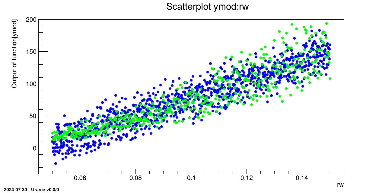
This file contains a MultiLinearFunction function. Comparison is made with a database generated from random variables obeying uniform laws and output variable calculated with this database and the MultiLinearFunction function.

"""
Example of multi-linear regression on flowrate
"""
from rootlogon import ROOT, DataServer, Launcher, Modeler, Sampler

tds = DataServer.TDataServer()
tds.fileDataRead("flowrate_sampler_launcher_500.dat")

c = ROOT.TCanvas("c1", "Graph for the Macro modeler", 5, 64, 1270, 667)
c.Divide(2)
c.cd(1)
tds.draw("yhat:rw")

# tds.getAttribute("yhat").setOutput()

tlin = Modeler.TLinearRegression(tds, "rw:r:tu:tl:hu:hl:l:kw",
                                 "yhat", "DummyForPython")
tlin.estimate()

tlin.exportFunction("c++", "_FileContainingFunction_", "MultiLinearFunction")

# Define the DataServer
tds2 = DataServer.TDataServer("tdsFlowrate", "Design of experiments")

# Add the study attributes
tds2.addAttribute(DataServer.TUniformDistribution("rw", 0.05, 0.15))
tds2.addAttribute(DataServer.TUniformDistribution("r", 100.0, 50000.0))
tds2.addAttribute(DataServer.TUniformDistribution("tu", 63070.0, 115600.0))
tds2.addAttribute(DataServer.TUniformDistribution("tl", 63.1, 116.0))
tds2.addAttribute(DataServer.TUniformDistribution("hu", 990.0, 1110.0))
tds2.addAttribute(DataServer.TUniformDistribution("hl", 700.0, 820.0))
tds2.addAttribute(DataServer.TUniformDistribution("l", 1120.0, 1680.0))
tds2.addAttribute(DataServer.TUniformDistribution("kw", 9855.0, 12045.0))

nS = 1000
# Generate DOE
sampling = Sampler.TSampling(tds2, "lhs", nS)
sampling.generateSample()

ROOT.gROOT.LoadMacro("_FileContainingFunction_.C")

# Create a TLauncherFunction from a TDataServer and an analytical function
# Rename the outpout attribute "ymod"
tlf = Launcher.TLauncherFunction(tds2, "MultiLinearFunction", "", "ymod")
# Evaluate the function on all the design of experiments
tlf.run()

c.Clear()
tds2.getTuple().SetMarkerColor(ROOT.kBlue)
tds2.getTuple().SetMarkerStyle(8)
tds2.getTuple().SetMarkerSize(1.2)

tds.getTuple().SetMarkerColor(ROOT.kGreen)
tds.getTuple().SetMarkerStyle(8)
tds.getTuple().SetMarkerSize(1.2)

tds2.draw("ymod:rw")
tds.draw("yhat:rw", "", "same")

The TDataServer is loaded with the database contained in the file flowrate_sampler_launcher_500.dat with the fileDataRead method:

tds = DataServer.TDataServer();
tds.fileDataRead("flowrate_sampler_launcher_500.dat");

The linear regression is initialised and characteristic values are computed for each variable with the estimate method:

tlin=Modeler.TLinearRegression(tds, "rw:r:tu:tl:hu:hl:l:kw", "yhat", "DummyForPython");
tlin.estimate();

The last argument is the option field, which in most cases is empty. Here it is filled with "DummyPython" which helps specify to python which constructor to choose. There are indeed several possible constructors these 5 five first arguments, but C++ can make the difference between them as the literal members are either std::string, ROOT::TString, Char_t* or even Option_t*. For python, these format are all PyString, so the sixth argument is compulsory to disentangle the possibilities.

The model is exported in an external file in C++ language _FileContainingFunction_.C where the function name is MultiLinearFunction:

tlin.exportFunction("c++", "_FileContainingFunction_", "MultiLinearFunction");

A second TDataServer is created. The previous variables then obey uniform laws and are linked as TAttribute in this new TDataServer:

tds2.addAttribute(DataServer.TUniformDistribution("rw", 0.05, 0.15));
tds2.addAttribute(DataServer.TUniformDistribution("r", 100.0, 50000.0));
tds2.addAttribute(DataServer.TUniformDistribution("tu", 63070.0, 115600.0));
tds2.addAttribute(DataServer.TUniformDistribution("tl", 63.1, 116.0));
tds2.addAttribute(DataServer.TUniformDistribution("hu", 990.0, 1110.0));
tds2.addAttribute(DataServer.TUniformDistribution("hl", 700.0, 820.0));
tds2.addAttribute(DataServer.TUniformDistribution("l", 1120.0, 1680.0));
tds2.addAttribute(DataServer.TUniformDistribution("kw", 9855.0, 12045.0));

A sampling is realised with a LHS method on 1000 patterns:

sampling = Sampler.TSampling(tds2, "lhs", nS);
sampling.generateSample();

The previously exported macro _FileContainingFunction_.C is loaded so as to perform calculation over the database in the second TDataServer with the function MultiLinearFunction. Results are stored in the ymod variable:

gROOT.LoadMacro("_FileContainingFunction_.C");
tlf=Launcher.TLauncherFunction(tds2, "MultiLinearFunction","","ymod");
tlf.run();

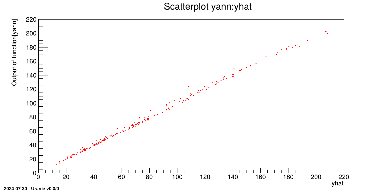
The objective of this macro is to build a surrogate model (an Artificial Neural Network) from a database. From a first database created from an ASCII file flowrate_sampler_launcher_500.dat (which defines values for eight variables described in Section IV.1.2.1 on 500 patterns), two ASCII files are created: one with the 300st patterns (_flowrate_sampler_launcher_app_.dat), the other with the 200 last patterns (_flowrate_sampler_launcher_val_.dat). The surrogate model is built with the database extracted from the first of the two files, the second allowing to perform calculations with a function.

"""
Example of neural network usage on flowrate
"""
from rootlogon import ROOT, DataServer, Launcher, Modeler

# Create a DataServer.TDataServer
# Load a database in an ASCII file
tdsu = DataServer.TDataServer("tdsu", "tds u")
tdsu.fileDataRead("flowrate_sampler_launcher_500.dat")

#
tdsu.exportData("_flowrate_sampler_launcher_app_.dat", "",
                "tdsFlowrate__n__iter__<=300")
tdsu.exportData("_flowrate_sampler_launcher_val_.dat", "",
                "tdsFlowrate__n__iter__>300")

tds = DataServer.TDataServer("tdsFlowrate", "tds for flowrate")
tds.fileDataRead("_flowrate_sampler_launcher_app_.dat")

c = ROOT.TCanvas("c1", "Graph for the Macro modeler", 5, 64, 1270, 667)
# Buils a surrogate model (Artificial Neural Networks) from the DataBase
tann = Modeler.TANNModeler(tds, "rw:r:tu:tl:hu:hl:l:kw, 3,yhat")
tann.setFcnTol(1e-5)
# tann.setLog()
tann.train(3, 2, "test")

tann.exportFunction("pmmlc++", "uranie_ann_flowrate", "ANNflowrate")

ROOT.gROOT.LoadMacro("uranie_ann_flowrate.C")

tdsv = DataServer.TDataServer()
tdsv.fileDataRead("_flowrate_sampler_launcher_val_.dat")

print(tdsv.getNPatterns())

# evaluate the surrogate model on the database
tlf = Launcher.TLauncherFunction(tdsv, "ANNflowrate",
                                 "rw:r:tu:tl:hu:hl:l:kw", "yann")
tlf.run()

tdsv.startViewer()

tdsv.Draw("yann:yhat")
# tdsv.draw("yhat")

The main TDataServer loads the main ASCII data file flowrate_sampler_launcher_500.dat

tdsu = DataServer.TDataServer("tdsu","tds u");
tdsu.fileDataRead("flowrate_sampler_launcher_500.dat");

The database is split in two parts by exporting the 300st patterns in a file and the remaining 200 in another one:

tdsu.exportData("_flowrate_sampler_launcher_app_.dat", "","tdsFlowrate__n__iter__<=300");
tdsu.exportData("_flowrate_sampler_launcher_val_.dat", "","tdsFlowrate__n__iter__>300");

A second TDataServer loads _flowrate_sampler_launcher_app_.dat and builds the surrogate model over all the variables:

tds = DataServer.TDataServer("tds", "tds for flowrate");
tds.fileDataRead("_flowrate_sampler_launcher_app_.dat");
tann=Modeler.TANNModeler(tds, "rw:r:tu:tl:hu:hl:l:kw,3,yhat"); 
tann.setFcnTol(1e-5);
tann.train(3, 2, "test");

The model is exported in an external file in C++ language "uranie_ann_flowrate.C where the function name is ANNflowrate:

tann.exportFunction("c++", "uranie_ann_flowrate","ANNflowrate");

The model is loaded from the macro "uranie_ann_flowrate.C and applied on the second database with the function ANNflowrate:

gROOT.LoadMacro("uranie_ann_flowrate.C");
tdsv = DataServer.TDataServer();
tdsv.fileDataRead("_flowrate_sampler_launcher_val_.dat");
tlf=Launcher.TLauncherFunction(tdsv, "ANNflowrate", "rw:r:tu:tl:hu:hl:l:kw", "yann");
tlf.run();

Processing modelerFlowrateNeuralNetworks.py...

--- Uranie v0.0/0 --- Developed with ROOT (6.32.02)
                      Copyright (C) 2013-2024 CEA/DES 
                      Contact: support-uranie@cea.fr 
                      Date: Tue Jan 09, 2024

 <URANIE::WARNING> 
 <URANIE::WARNING> *** URANIE WARNING ***
 <URANIE::WARNING> *** File[${SOURCEDIR}/dataSERVER/souRCE/TDataServer.cxx] Line[759]
 <URANIE::WARNING> TDataServer::fileDataRead: Expected iterator tdsu__n__iter__ not found but tdsFlowrate__n__iter__ looks like an URANIE iterator => Will be used as so.
 <URANIE::WARNING> *** END of URANIE WARNING ***
 <URANIE::WARNING> 
 ** TANNModeler::train niter[3] ninit[2]
 ** init the ANN
 ** Input  (1) Name[rw] Min[0.101018] Max[0.0295279]
 ** Input  (2) Name[r] Min[25668.6] Max[14838.3]
 ** Input  (3) Name[tu] Min[89914.4] Max[14909]
 ** Input  (4) Name[tl] Min[89.0477] Max[15.0121]
 ** Input  (5) Name[hu] Min[1048.92] Max[34.8615]
 ** Input  (6) Name[hl] Min[763.058] Max[33.615]
 ** Input  (7) Name[l] Min[1401.09] Max[163.611]
 ** Input  (8) Name[kw] Min[10950.2] Max[635.503]
 ** Output  (1) Name[yhat] Min[78.0931] Max[44.881]
 ** Tolerance  (1e-05)
 ** sHidden    (3) (3)
 ** Nb Weights (31)
 ** ActivationFunction[LOGISTIC]
 **

 ** iter[1/3] : *= : mse_min[0.00150425]
 ** iter[2/3] : ** : mse_min[0.0024702]
 ** iter[3/3] : *= : mse_min[0.00122167]

 ** solutions : 3
 ** isol[1] iter[0] learn[0.00126206] test[0.00150425] *
 ** isol[2] iter[1] learn[0.00152949] test[0.0024702]
 ** isol[3] iter[2] learn[0.00107926] test[0.00122167] *
 ** CPU training finished. Total elapsed time: 1.5 sec

*******************************
*** TModeler::exportFunction lang[pmmlc++] file[uranie_ann_flowrate] name[ANNflowrate] soption[]

*******************************

*******************************
*** exportFunction lang[pmmlc++] file[uranie_ann_flowrate] name[ANNflowrate]

*******************************
PMML Constructor: uranie_ann_flowrate.pmml
*** End Of exportModelPMML 
*******************************
*** End Of exportFunction
*******************************

The objective of this macro is to build a surrogate model (an Artificial Neural Network) from a PMML file.

"""
Example of neural network loaded from pmml for flowrate
"""
from rootlogon import ROOT, DataServer, Launcher, Modeler

# Create a DataServer.TDataServer
# Load a database in an ASCII file
tds = DataServer.TDataServer("tdsFlowrate", "tds for flowrate")
tds.fileDataRead("_flowrate_sampler_launcher_app_.dat")

c = ROOT.TCanvas("c1", "Graph for the Macro modeler", 5, 64, 1270, 667)
# Build a surrogate model (Artificial Neural Networks) from the PMML file
tann = Modeler.TANNModeler(tds, "uranie_ann_flowrate.pmml", "ANNflowrate")

# export the surrogate model in a C file
tann.exportFunction("c++", "uranie_ann_flowrate_loaded", "ANNflowrate")
# load the surrogate model in the C file
ROOT.gROOT.LoadMacro("uranie_ann_flowrate_loaded.C")

tdsv = DataServer.TDataServer("tdsv", "tds for surrogate model")
tdsv.fileDataRead("_flowrate_sampler_launcher_val_.dat")

print(tdsv.getNPatterns())

# evaluate the surrogate model on the database
tlf = Launcher.TLauncherFunction(tdsv, "ANNflowrate",
                                 "rw:r:tu:tl:hu:hl:l:kw", "yann")
tlf.run()

tdsv.startViewer()

tdsv.Draw("yann:yhat")
# tdsv.draw("yhat")

A TDataServer loads _flowrate_sampler_launcher_app_.dat:

tds = DataServer.TDataServer("tds", "tds for flowrate");
tds.fileDataRead("_flowrate_sampler_launcher_app_.dat");

The surrogate model is loaded from a PMML file:

tann=Modeler.TANNModeler(tds, "uranie_ann_flowrate.pmml","ANNflowrate");

The model is exported in an external file in C++ language "uranie_ann_flowrate where the function name is ANNflowrate:

tann.exportFunction("c++", "uranie_ann_flowrate","ANNflowrate");

The model is loaded from the macro "uranie_ann_flowrate.C and applied on the database with the function ANNflowrate:

gROOT.LoadMacro("uranie_ann_flowrate.C");
tdsv = DataServer.TDataServer();
tdsv.fileDataRead("_flowrate_sampler_launcher_val_.dat");
tlf=Launcher.TLauncherFunction(tdsv, "ANNflowrate", "rw:r:tu:tl:hu:hl:l:kw", "yann");
tlf.run();

Processing modelerFlowrateNeuralNetworksLoadingPMML.py...

--- Uranie v0.0/0 --- Developed with ROOT (6.32.02)
                      Copyright (C) 2013-2024 CEA/DES 
                      Contact: support-uranie@cea.fr 
                      Date: Tue Jan 09, 2024

PMML Constructor: uranie_ann_flowrate.pmml

*******************************
*** TModeler::exportFunction lang[c++] file[uranie_ann_flowrate_loaded] name[ANNflowrate] soption[]

*******************************

*******************************
*** exportFunction lang[c++] file[uranie_ann_flowrate_loaded] name[ANNflowrate]
*** End Of exportFunction
*******************************

The objective of this macro is to build a surrogate model (an Artificial Neural Network) from a database for a "Classification" Problem. From a first database loaded from the ASCII file problem2Classes_001000.dat, which defines three variables 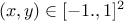and on 1000 patterns,

two ASCII files are created, one with the 800st patterns (_problem2Classes_app_.dat), the other with the 200 last patterns (_problem2Classes_val_.dat). The surrogate model is built with the database extracted from the first of the two files, the second allowing to perform calculations with a function.

"""
Example of classification problem with neural network
"""
from rootlogon import ROOT, DataServer, Launcher, Modeler

nH1 = 15
nH2 = 10
nH3 = 5

sX = "x:y"
sY = "rc01"
sYhat = sY+"_"+str(nH1)+"_"+str(nH2)+"_"+str(nH3)

# Load a database in an ASCII file
tdsu = DataServer.TDataServer("tdsu", "tds u")
tdsu.fileDataRead("problem2Classes_001000.dat")

# Split into 2 datasets for learning and testing
Niter = tdsu.getIteratorName()
tdsu.exportData("_problem2Classes_app_.dat", "", Niter+"<=800")
tdsu.exportData("_problem2Classes_val_.dat", "", Niter+">800")

tds = DataServer.TDataServer("tdsApp", "tds App for problem2Classes")
tds.fileDataRead("_problem2Classes_app_.dat")

tann = Modeler.TANNModeler(tds, sX+", %i, %i, %i,@" % (nH1, nH2, nH3)+sY)
# tann.setLog()
tann.setNormalization(Modeler.TANNModeler.kMinusOneOne)
tann.setFcnTol(1e-6)
tann.train(2, 2, "test", False)

tann.exportFunction("c++", "uranie_ann_problem2Classes", "ANNproblem2Classes")

ROOT.gROOT.LoadMacro("uranie_ann_problem2Classes.C")

tdsv = DataServer.TDataServer()
tdsv.fileDataRead("_problem2Classes_val_.dat")

# evaluate the surrogate model on the database
tlf = Launcher.TLauncherFunction(tdsv, "ANNproblem2Classes", sX, sYhat)
tlf.run()

c = ROOT.TCanvas("c1", "Graph for the Macro modeler", 5, 64, 1270, 667)
# Buils a surrogate model (Artificial Neural Networks) from the DataBase
tds.getTuple().SetMarkerStyle(8)
tds.getTuple().SetMarkerSize(1.0)
tds.getTuple().SetMarkerColor(ROOT.kGreen)
tds.draw(sY+":"+sX)

tdsv.getTuple().SetMarkerStyle(8)
tdsv.getTuple().SetMarkerSize(0.75)
tdsv.getTuple().SetMarkerColor(ROOT.kRed)
tdsv.Draw(sYhat+":"+sX, "", "same")

The main TDataServer loads the main ASCII data file problem2Classes_001000.dat

tdsu = DataServer.TDataServer("tdsu","tds u");
tdsu.fileDataRead("problem2Classes_001000.dat");

The database is split with the internal iterator attribute in two parts by exporting the 800st patterns in a file and the remaining 200 in another one

tdsu.exportData("_problem2Classes_app_.dat", "",Form("%s<=800", tdsu.getIteratorName()));
tdsu.exportData("_problem2Classes_val_.dat", "", Form("%s>800", tdsu.getIteratorName()));

A second TDataServer loads _problem2Classes_app_.dat and builds the surrogate model over all the variables with 3 hidden layers, a Hyperbolic Tangent (TanH) activation function (normalization) in the 3 hidden layers and set the function tolerance to 1e-.6. The "@" character behind the output name defines a classification problem.

tds = DataServer.TDataServer("tds", "tds for the 2 Classes problem");
tds.fileDataRead("_problem2Classes_app_.dat");
tann=Modeler.TANNModeler(tds, sX+","+str(nH1)+","+str(nH2)+","+str(nH3)+",@"+sY); 
tann.setNormalization(Modeler.TANNModeler.kMinusOneOne)
tann.setFcnTol(1e-6);
tann.train(3, 2, "test");

The model is exported in an external file in C++ language "uranie_ann_problem2Classes.C" where the function name is ANNproblem2Classes

tann.exportFunction("c++", "uranie_ann_problem2Classes","ANNproblem2Classes");

The model is loaded from the macro "uranie_ann_problem2Classes.C and applied on the second database with the function ANNproblem2Classes.

gROOT.LoadMacro("uranie_ann_problem2Classes.C");
tdsv = DataServer.TDataServer();
tdsv.fileDataRead("_problem2Classes_val_.dat");
tlf=Launcher.TLauncherFunction(tdsv, "ANNproblem2Classes", sX, sYhat);
tlf.run();

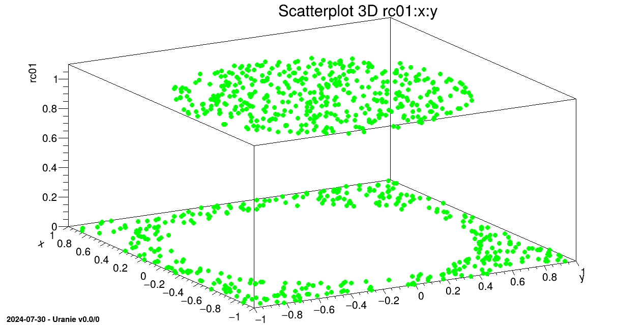
We draw on a 3D graph, the learning database (in green) and the estimations by the Artificial Neural Network with red points.

c=ROOT.TCanvas("c1", "Graph for the Macro modeler",5,64,1270,667);
tds.getTuple().SetMarkerStyle(8);
tds.getTuple().SetMarkerSize(1.0);
tds.getTuple().SetMarkerColor(kGreen);
tds.draw(Form("%s:%s", sY.Data(), sX.Data()));

tdsv.getTuple().SetMarkerStyle(8);
tdsv.getTuple().SetMarkerSize(0.75);
tdsv.getTuple().SetMarkerColor(kRed);
tdsv.Draw(Form("%s:%s", sYhat.Data(), sX.Data()),"","same");
	

Processing modelerClassificationNeuralNetworks.py...

--- Uranie v0.0/0 --- Developed with ROOT (6.32.02)
                      Copyright (C) 2013-2024 CEA/DES 
                      Contact: support-uranie@cea.fr 
                      Date: Tue Jan 09, 2024

 <URANIE::WARNING> 
 <URANIE::WARNING> *** URANIE WARNING ***
 <URANIE::WARNING> *** File[${SOURCEDIR}/dataSERVER/souRCE/TDataServer.cxx] Line[759]
 <URANIE::WARNING> TDataServer::fileDataRead: Expected iterator tdsu__n__iter__ not found but _tds___n__iter__ looks like an URANIE iterator => Will be used as so.
 <URANIE::WARNING> *** END of URANIE WARNING ***
 <URANIE::WARNING> 
 <URANIE::WARNING> 
 <URANIE::WARNING> *** URANIE WARNING ***
 <URANIE::WARNING> *** File[${SOURCEDIR}/dataSERVER/souRCE/TDataServer.cxx] Line[759]
 <URANIE::WARNING> TDataServer::fileDataRead: Expected iterator tdsApp__n__iter__ not found but _tds___n__iter__ looks like an URANIE iterator => Will be used as so.
 <URANIE::WARNING> *** END of URANIE WARNING ***
 <URANIE::WARNING> 
 ** TANNModeler::train niter[2] ninit[2]
 ** init the ANN
 ** Input  (1) Name[x] Min[-0.999842] Max[0.998315]
 ** Input  (2) Name[y] Min[-0.999434] Max[0.998071]
 ** Output  (1) Name[rc01] Min[0] Max[1]
 ** Tolerance  (1e-06)
 ** sHidden    (15,10,5) (30)
 ** Nb Weights (266)
 ** ActivationFunction[TanH]
 **

 ** iter[1/2] : ** : mse_min[0.00813999]
 ** iter[2/2] : ** : mse_min[0.00636923]

 ** solutions : 2
 ** isol[1] iter[0] learn[0.00405863] test[0.00813999] *
 ** isol[2] iter[1] learn[0.00560685] test[0.00636923] *
 ** CPU training finished. Total elapsed time: 16.8 sec

*******************************
*** TModeler::exportFunction lang[c++] file[uranie_ann_problem2Classes] name[ANNproblem2Classes] soption[]

*******************************

*******************************
*** exportFunction lang[c++] file[uranie_ann_problem2Classes] name[ANNproblem2Classes]
*** End Of exportFunction
*******************************

The objective of this macro is to build a polynomial chaos expansion in order to get a surrogate model along with a global sensitivity interpretation for the flowrate function, whose purpose and behaviour have been already introduced in Section IV.1.2.1. The method used here is the regression one, as discussed below.

"""
Example of Chaos polynomial expansion using regression estimation on flowrate
"""
from rootlogon import ROOT, DataServer, Launcher, Modeler

ROOT.gROOT.LoadMacro("UserFunctions.C")

# Define the DataServer
tds = DataServer.TDataServer("tdsflowreate", "DataBase flowreate")
tds.addAttribute(DataServer.TUniformDistribution("rw", 0.05, 0.15))
tds.addAttribute(DataServer.TUniformDistribution("r", 100.0, 50000.0))
tds.addAttribute(DataServer.TUniformDistribution("tu", 63070.0, 115600.0))
tds.addAttribute(DataServer.TUniformDistribution("tl", 63.1, 116.0))
tds.addAttribute(DataServer.TUniformDistribution("hu", 990.0, 1110.0))
tds.addAttribute(DataServer.TUniformDistribution("hl", 700.0, 820.0))
tds.addAttribute(DataServer.TUniformDistribution("l", 1120.0, 1680.0))
tds.addAttribute(DataServer.TUniformDistribution("kw", 9855.0, 12045.0))

# Define of TNisp object
nisp = Modeler.TNisp(tds)
nisp.generateSample("QmcSobol", 500)  # State that there is a sample ...

# Compute the output variable
tlf = Launcher.TLauncherFunction(tds, "flowrateModel", "*", "ymod")
tlf.setDrawProgressBar(False)
tlf.run()

# build a chaos polynomial
pc = Modeler.TPolynomialChaos(tds, nisp)

# compute the pc coefficients using the "Regression" method
degree = 4
pc.setDegree(degree)
pc.computeChaosExpansion("Regression")

# Uncertainty and sensitivity analysis
print("Variable ymod ================")
print("Mean     = "+str(pc.getMean("ymod")))
print("Variance = "+str(pc.getVariance("ymod")))
print("First Order Indices ================")
print("Indice First Order[1] = "+str(pc.getIndexFirstOrder(0, 0)))
print("Indice First Order[2] = "+str(pc.getIndexFirstOrder(1, 0)))
print("Indice First Order[3] = "+str(pc.getIndexFirstOrder(2, 0)))
print("Indice First Order[4] = "+str(pc.getIndexFirstOrder(3, 0)))
print("Indice First Order[5] = "+str(pc.getIndexFirstOrder(4, 0)))
print("Indice First Order[6] = "+str(pc.getIndexFirstOrder(5, 0)))
print("Indice First Order[7] = "+str(pc.getIndexFirstOrder(6, 0)))
print("Indice First Order[8] = "+str(pc.getIndexFirstOrder(7, 0)))
print("Total Order Indices ================")
print("Indice Total Order[1] = "+str(pc.getIndexTotalOrder("rw", "ymod")))
print("Indice Total Order[2] = "+str(pc.getIndexTotalOrder("r", "ymod")))
print("Indice Total Order[3] = "+str(pc.getIndexTotalOrder("tu", "ymod")))
print("Indice Total Order[4] = "+str(pc.getIndexTotalOrder("tl", "ymod")))
print("Indice Total Order[5] = "+str(pc.getIndexTotalOrder("hu", "ymod")))
print("Indice Total Order[6] = "+str(pc.getIndexTotalOrder("hl", "ymod")))
print("Indice Total Order[7] = "+str(pc.getIndexTotalOrder("l", "ymod")))
print("Indice Total Order[8] = "+str(pc.getIndexTotalOrder("kw", "ymod")))

# Dump main factors up to a certain threshold
seuil = 0.99
print("Ordered functionnal ANOVA")
pc.getAnovaOrdered(seuil, 0)

print("Number of experiments = "+str(tds.getNPatterns()))

# save the pv in a program (C langage)
pc.exportFunction("NispFlowrate", "NispFlowrate")

The first part is just creating a TDataServer and providing the attributes needed to define the problem. From there, a TNisp object is created, providing the dataserver that specifies the inputs. This class is used to generate the sample.

# Define of TNisp object
nisp=Modeler.TNisp(tds);
nisp.generateSample("QmcSobol", 500); #State that there is a sample ...

The function is launched through a TLauncherFunction instance in order to get the output values that will be needed to train the surrogate model.

tlf=Launcher.TLauncherFunction(tds, "flowrateModel","*","ymod");
tlf.run();

Finally, a TPolynomialChaos instance is created and the computation of the coefficients is performed by requesting a truncature on the resulting degree of the polynomial expansion (set to 4) and the use of a regression method.

pc=Modeler.TPolynomialChaos(tds,nisp); 
# compute the pc coefficients using the "Regression" method
degree = 4;
pc.setDegree(degree);
pc.computeChaosExpansion("Regression");

The rest of the code is showing how to access the resulting sensitivity indices either one-by-one, or ordered up to a chosen threshold of the output variance.

Processing modelerFlowratePolynChaosRegression.py...

--- Uranie v0.0/0 --- Developed with ROOT (6.32.02)
                      Copyright (C) 2013-2024 CEA/DES 
                      Contact: support-uranie@cea.fr 
                      Date: Tue Jan 09, 2024

Variable ymod ================
Mean     = 77.6510221869
Variance = 2079.68093305
First Order Indices ================
Indice First Order[1] = 0.828731527534
Indice First Order[2] = 1.05548253583e-06
Indice First Order[3] = 9.86804533168e-08
Indice First Order[4] = 4.77668083154e-06
Indice First Order[5] = 0.0414014932666
Indice First Order[6] = 0.041321536203
Indice First Order[7] = 0.0394009661592
Indice First Order[8] = 0.00954643619285
Total Order Indices ================
Indice Total Order[1] = 0.86677277638
Indice Total Order[2] = 9.2746650823e-06
Indice Total Order[3] = 7.01768059052e-06
Indice Total Order[4] = 1.71943739446e-05
Indice Total Order[5] = 0.054191575612
Indice Total Order[6] = 0.0540578172024
Indice Total Order[7] = 0.0522121155838
Indice Total Order[8] = 0.0127808734357

The objective of this macro is to build a polynomial chaos expansion in order to get a surrogate model along with a global sensitivity interpretation for the flowrate function, whose purpose and behaviour have been already introduced in Section IV.1.2.1. The method used here is the regression one, as discussed below.

"""
Example of Chaos polynomial expansion on flowrate
"""
from rootlogon import ROOT, DataServer, Launcher, Modeler

ROOT.gROOT.LoadMacro("UserFunctions.C")

# Define the DataServer
tds = DataServer.TDataServer("tdsflowreate", "DataBase flowreate")
tds.addAttribute(DataServer.TUniformDistribution("rw", 0.05, 0.15))
tds.addAttribute(DataServer.TUniformDistribution("r", 100.0, 50000.0))
tds.addAttribute(DataServer.TUniformDistribution("tu", 63070.0, 115600.0))
tds.addAttribute(DataServer.TUniformDistribution("tl", 63.1, 116.0))
tds.addAttribute(DataServer.TUniformDistribution("hu", 990.0, 1110.0))
tds.addAttribute(DataServer.TUniformDistribution("hl", 700.0, 820.0))
tds.addAttribute(DataServer.TUniformDistribution("l", 1120.0, 1680.0))
tds.addAttribute(DataServer.TUniformDistribution("kw", 9855.0, 12045.0))

# Define of TNisp object
nisp = Modeler.TNisp(tds)
nisp.generateSample("Petras", 5)  # State that there is a sample ...

# Compute the output variable
tlf = Launcher.TLauncherFunction(tds, "flowrateModel", "*", "ymod")
tlf.setDrawProgressBar(False)
tlf.run()

# build a chaos polynomial
pc = Modeler.TPolynomialChaos(tds, nisp)

# compute the pc coefficients using the "Integration" method
degree = 4
pc.setDegree(degree)
pc.computeChaosExpansion("Integration")

# Uncertainty and sensitivity analysis
print("Variable ymod ================")
print("Mean     = "+str(pc.getMean("ymod")))
print("Variance = "+str(pc.getVariance("ymod")))
print("First Order Indices ================")
print("Indice First Order[1] = "+str(pc.getIndexFirstOrder(0, 0)))
print("Indice First Order[2] = "+str(pc.getIndexFirstOrder(1, 0)))
print("Indice First Order[3] = "+str(pc.getIndexFirstOrder(2, 0)))
print("Indice First Order[4] = "+str(pc.getIndexFirstOrder(3, 0)))
print("Indice First Order[5] = "+str(pc.getIndexFirstOrder(4, 0)))
print("Indice First Order[6] = "+str(pc.getIndexFirstOrder(5, 0)))
print("Indice First Order[7] = "+str(pc.getIndexFirstOrder(6, 0)))
print("Indice First Order[8] = "+str(pc.getIndexFirstOrder(7, 0)))
print("Total Order Indices ================")
print("Indice Total Order[1] = "+str(pc.getIndexTotalOrder("rw", "ymod")))
print("Indice Total Order[2] = "+str(pc.getIndexTotalOrder("r", "ymod")))
print("Indice Total Order[3] = "+str(pc.getIndexTotalOrder("tu", "ymod")))
print("Indice Total Order[4] = "+str(pc.getIndexTotalOrder("tl", "ymod")))
print("Indice Total Order[5] = "+str(pc.getIndexTotalOrder("hu", "ymod")))
print("Indice Total Order[6] = "+str(pc.getIndexTotalOrder("hl", "ymod")))
print("Indice Total Order[7] = "+str(pc.getIndexTotalOrder("l", "ymod")))
print("Indice Total Order[8] = "+str(pc.getIndexTotalOrder("kw", "ymod")))

# Dump main factors up to a certain threshold
seuil = 0.99
print("Ordered functionnal ANOVA")
pc.getAnovaOrdered(seuil, 0)

print("Number of experiments = "+str(tds.getNPatterns()))

# save the pv in a program (C langage)
pc.exportFunction("NispFlowrate", "NispFlowrate")

The first part is just creating a TDataServer and providing the attributes needed to define the problem. From there, a TNisp object is created, providing the dataserver that specifies the inputs. This class is used to generate the sample (Petras being a design-of-experiments dedicated to integration problem).

nisp=Modeler.TNisp(tds);
nisp.generateSample("Petras", 5); #State that there is a sample ...

The function is launched through a TLauncherFunction instance in order to get the output values that will be needed to train the surrogate model.

tlf=Launcher.TLauncherFunction(tds, "flowrateModel","*","ymod");
tlf.run();

Finally, a TPolynomialChaos instance is created and the computation of the coefficients is performed by requesting a truncature on the resulting degree of the polynomial expansion (set to 4) and the use of a regression method.

pc=Modeler.TPolynomialChaos(tds,nisp); 
# compute the pc coefficients using the "Integration" method
degree = 4;
pc.setDegree(degree);
pc.computeChaosExpansion("Integration");

The rest of the code is showing how to access the resulting sensitivity indices either one-by-one, or ordered up to a chosen threshold of the output variance.

Processing modelerFlowratePolynChaosIntegration.py...

--- Uranie v0.0/0 --- Developed with ROOT (6.32.02)
                      Copyright (C) 2013-2024 CEA/DES 
                      Contact: support-uranie@cea.fr 
                      Date: Tue Jan 09, 2024

Variable ymod ================
Mean     = 77.6510994117
Variance = 2078.9066967
First Order Indices ================
Indice First Order[1] = 0.828922140066
Indice First Order[2] = 1.04476604502e-06
Indice First Order[3] = 8.94692085494e-12
Indice First Order[4] = 5.30298679946e-06
Indice First Order[5] = 0.0413851874777
Indice First Order[6] = 0.0413851874777
Indice First Order[7] = 0.0393418959892
Indice First Order[8] = 0.00952157178884
Total Order Indices ================
Indice Total Order[1] = 0.866833983627
Indice Total Order[2] = 2.16178081947e-06
Indice Total Order[3] = 2.28296199168e-09
Indice Total Order[4] = 1.07385825248e-05
Indice Total Order[5] = 0.0541095486382
Indice Total Order[6] = 0.0541095486382
Indice Total Order[7] = 0.0520766679067
Indice Total Order[8] = 0.0127305987998

This macro is the one described in Section V.6.2.2, that creates a simple gaussian process, whose training (utf_4D_train.dat) and testing (utf_4D_test.dat) database can both be found in the document folder of the Uranie installation (${URANIESYS}/share/uranie/docUMENTS).

"""
Example of Gaussian Process building
"""
from rootlogon import DataServer, Modeler

# Load observations
tdsObs = DataServer.TDataServer("tdsObs", "observations")
tdsObs.fileDataRead("utf_4D_train.dat")

# Construct the GPBuilder
gpb = Modeler.TGPBuilder(tdsObs,         # observations data
                         "x1:x2:x3:x4",  # list of input variables
                         "y",            # output variable
                         "matern3/2")    # name of the correlation function


# Search for the optimal hyper-parameters
gpb.findOptimalParameters("ML",          # optimisation criterion
                          100,           # screening design size
                          "neldermead",  # optimisation algorithm
                          500)           # max. number of optim iterations

# Construct the kriging model
krig = gpb.buildGP()

# Display model information
krig.printLog()

This is the result of the last command:

*******************************
** TKriging::printLog[]
*******************************
 Input Variables:      x1:x2:x3:x4
 Output Variable:      y
 Deterministic trend:  
 Correlation function: URANIE::Modeler::TMatern32CorrFunction
 Correlation length:   normalised   (not normalised)
                       1.6181e+00 (1.6172e+00 )
                       1.4372e+00 (1.4370e+00 )
                       1.5026e+00 (1.5009e+00 )
                       6.7884e+00 (6.7944e+00 )

 Variance of the gaussian process:      70.8755
 RMSE (by Leave One Out):               0.499108
 Q2:                                    0.849843
*******************************

This macro is the one described in Section V.6.2.7, that creates a gaussian process, whose training (utf_4D_train.dat) and testing (utf_4D_test.dat) database can both be found in the document folder of the Uranie installation (${URANIESYS}/share/uranie/docUMENTS), and whose starting point, in the parameter space, is specified.

"""
Example of Gaussian Process building with initial point set
"""
import numpy as np
from rootlogon import DataServer, Modeler

# Load observations
tdsObs = DataServer.TDataServer("tdsObs", "observations")
tdsObs.fileDataRead("utf_4D_train.dat")

# Construct the GPBuilder
gpb = Modeler.TGPBuilder(tdsObs, "x1:x2:x3:x4", "y", "matern3/2")

# Set the correlation function parameters
params = np.array([1.0, 0.25, 0.01, 0.3])
gpb.getCorrFunction().setParameters(params)

# Find the optimal parameters
gpb.findOptimalParameters("ML",          # optimisation criterion
                          0,             # screening size MUST be equal to 0
                          "neldermead",  # optimisation algorithm
                          500,           # max. number of optim iterations
                          False)         # Don't reset parameters of GP builder

# Create the kriging model
krig = gpb.buildGP()

# Display model information
krig.printLog()

This is the result of the last command:

*******************************
** TKriging::printLog[]
*******************************
 Input Variables:      x1:x2:x3:x4
 Output Variable:      y
 Deterministic trend:  
 Correlation function: URANIE::Modeler::TMatern32CorrFunction
 Correlation length:   normalised   (not normalised)
                       1.6182e+00 (1.6173e+00 )
                       1.4373e+00 (1.4371e+00 )
                       1.5027e+00 (1.5011e+00 )
                       6.7895e+00 (6.7955e+00 )

 Variance of the gaussian process:      70.8914
 RMSE (by Leave One Out):               0.49911
 Q2:                                    0.849842
*******************************

This macro is the one described in Section V.6.2.4, that creates a gaussian process with a specific trend and an a priori knowledge on the mean and variance of the trend parameters.

"""
Example of Gaussian Process building with a priori knowledge
"""
import numpy as np
from rootlogon import DataServer, Modeler

# Load observations
tdsObs = DataServer.TDataServer("tdsObs", "observations")
tdsObs.fileDataRead("utf_4D_train.dat")

# Construct the GPBuilder
gpb = Modeler.TGPBuilder(tdsObs,         # observations data
                         "x1:x2:x3:x4",  # list of input variables
                         "y",            # output variable
                         "matern3/2",    # name of the correlation function
                         "linear")       # trend defined by a keyword

# Bayesian study
meanPrior = np.array([0.0, 0.0, -1.0, 0.0, -0.1])
covPrior = np.array([1e-4, 0.0, 0.0, 0.0, 0.0,
                     0.0, 1e-4, 0.0, 0.0, 0.0,
                     0.0, 0.0, 1e-4, 0.0, 0.0,
                     0.0, 0.0, 0.0, 1e-4, 0.0,
                     0.0, 0.0, 0.0, 0.0, 1e-4])
gpb.setPriorData(meanPrior, covPrior)

# Search for the optimal hyper-parameters
gpb.findOptimalParameters("ReML",        # optimisation criterion
                          100,           # screening design size
                          "neldermead",  # optimisation algorithm
                          500)           # max. number of optim iterations

# Construct the kriging model
krig = gpb.buildGP()

# Display model information
krig.printLog()

This is the result of the last command:

*******************************
** TKriging::printLog[]
*******************************
 Input Variables:      x1:x2:x3:x4
 Output Variable:      y
 Deterministic trend:  linear
 Trend parameters (5): [3.06586494e-05; 1.64887174e-05; -9.99986787e-01; 1.51959859e-05; -9.99877606e-02 ]
 Correlation function: URANIE::Modeler::TMatern32CorrFunction
 Correlation length:   normalised   (not normalised)
                       2.1450e+00 (2.1438e+00 )
                       1.9092e+00 (1.9090e+00 )
                       2.0062e+00 (2.0040e+00 )
                       8.4315e+00 (8.4390e+00 )

 Variance of the gaussian process:      155.533
 RMSE (by Leave One Out):               0.495448
 Q2:                                    0.852037
*******************************

This macro is the one described in Section V.6.3, to create and use a simple gaussian process, whose training (utf_4D_train.dat) and testing (utf_4D_test.dat) database can both be found in the document folder of the Uranie installation (${URANIESYS}/share/uranie/docUMENTS). It uses the simple one-by-one approch described in the [metho] for completness.

"""
Example of Gaussian Process building with estimation on another dataset
"""
from rootlogon import DataServer, Modeler, Relauncher

# Load observations
tdsObs = DataServer.TDataServer("tdsObs", "observations")
tdsObs.fileDataRead("utf_4D_train.dat")

# Construct the GPBuilder
gpb = Modeler.TGPBuilder(tdsObs,         # observations data
                         "x1:x2:x3:x4",  # list of input variables
                         "y",            # output variable
                         "matern3/2")    # name of the correlation function


# Search for the optimal hyper-parameters
gpb.findOptimalParameters("ML",          # optimisation criterion
                          100,           # screening design size
                          "neldermead",  # optimisation algorithm
                          500)           # max. number of optim iterations

# Construct the kriging model
krig = gpb.buildGP()

# Display model information
krig.printLog()

# Load the data to estimate
tdsEstim = DataServer.TDataServer("tdsEstim", "estimations")
tdsEstim.fileDataRead("utf_4D_test.dat")

# Construction of the launcher
lanceur = Relauncher.TLauncher2(tdsEstim,         # data to estimate
                                krig,             # model used
                                "x1:x2:x3:x4",    # list of the input variables
                                "yEstim:vEstim")  # name of model's outputs

# Launch the estimations
lanceur.solverLoop()

# Display some results
tdsEstim.draw("yEstim:y")

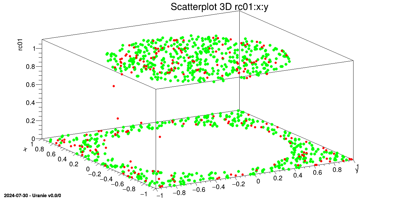
This macro is the one described in Section V.6.3.2, to create and use a simple gaussian process, whose training (utf_4D_train.dat) and testing (utf_4D_test.dat) database can both be found in the document folder of the Uranie installation (${URANIESYS}/share/uranie/docUMENTS). It uses the global approach, computing the input covariance matrix and translating it to the prediction covariance matrix.

"""
Example of Gaussian Process building with estimation using full data (covariance)
"""
from rootlogon import ROOT, DataServer, Modeler

# Load observations
tdsObs = DataServer.TDataServer("tdsObs", "observations")
tdsObs.fileDataRead("utf_4D_train.dat")

# Construct the GPBuilder
gpb = Modeler.TGPBuilder(tdsObs,         # observations data
                         "x1:x2:x3:x4",  # list of input variables
                         "y",            # output variable
                         "matern1/2")    # name of the correlation function


# Search for the optimal hyper-parameters
gpb.findOptimalParameters("ML",          # optimisation criterion
                          100,           # screening design size
                          "neldermead",  # optimisation algorithm
                          500)           # max. number of optim iterations

# Construct the kriging model
krig = gpb.buildGP()

# Display model information
krig.printLog()

# Load the data to estimate
tdsEstim = DataServer.TDataServer("tdsEstim", "estimations")
tdsEstim.fileDataRead("utf_4D_test.dat")

# Reducing DB to 1000 first event (leading to cov matrix of a million value)
nS = 1000
tdsEstim.exportData("utf_4D_test_red.dat", "", "tdsEstim__n__iter__<="+str(nS))
# Reload reduced sample
tdsEstim.fileDataRead("utf_4D_test_red.dat", False, True)

krig.estimateWithCov(tdsEstim,         # data to estimate
                     "x1:x2:x3:x4",    # list of the input variables
                     "yEstim:vEstim",  # name given to the model's outputs
                     "y",              # name of the true reference
                     "DummyOption")    # options

cTwo = None
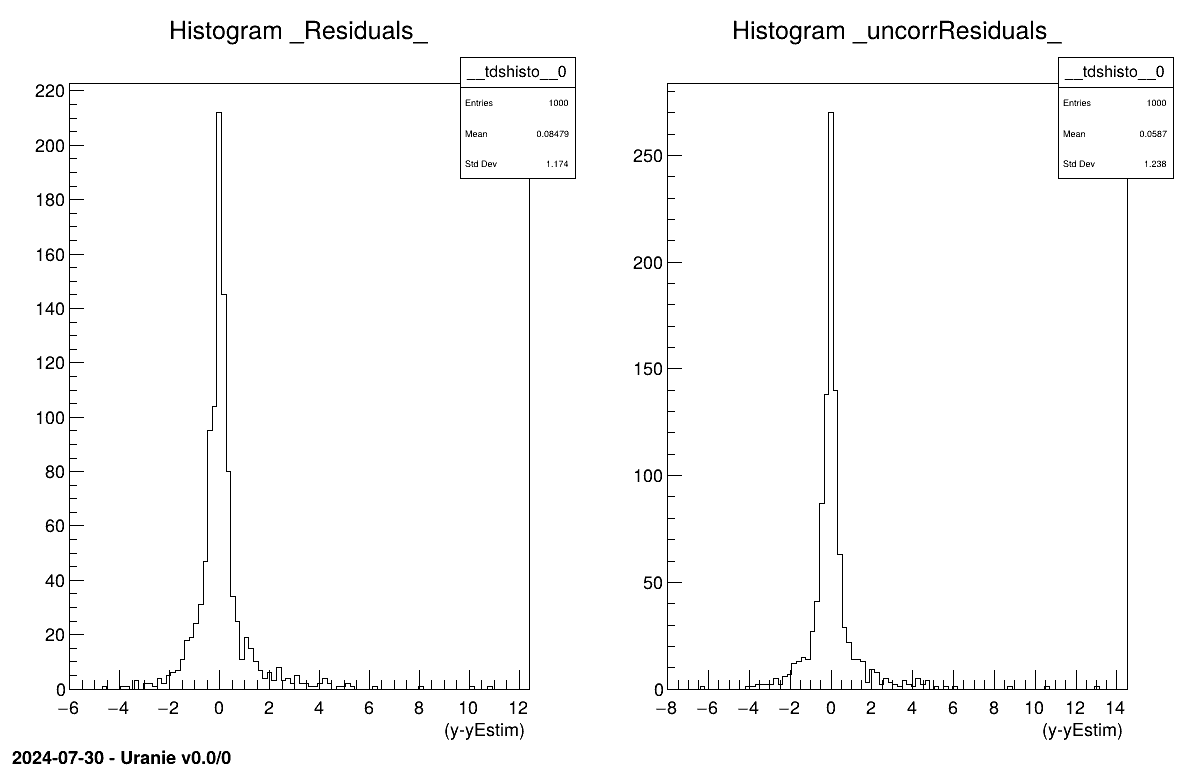
# Produce residuals plots if true information provided
if tdsEstim.isAttribute("_Residuals_"):
    cTwo = ROOT.TCanvas("c2", "c2", 1200, 800)
    cTwo.Divide(2, 1)
    cTwo.cd(1)
    # Usual residual considering uncorrated input points
    tdsEstim.Draw("_Residuals_")
    cTwo.cd(2)
    # Corrected residuals, taking full prediction covariance matrix
    tdsEstim.Draw("_uncorrResiduals_")

# Retrieve all the prediction covariance coefficient
tdsEstim.getTuple().SetEstimate(nS*nS)  # allocate the correct size
# Get a pointer to all values
tdsEstim.getTuple().Draw("_CovarianceMatrix_", "", "goff")
cov = tdsEstim.getTuple().GetV1()

# Put these in a matrix nicely created
Cov = ROOT.TMatrixD(nS, nS)
Cov.Use(0, nS-1, 0, nS-1, cov)

# Print it if size is reasonnable
if nS < 10:
    Cov.Print()

The idea is to provide a simple example of a kriging usage, and an how to, to produce plots in one dimension to represent the results. This example is the one taken from [metho] that uses a very simple set of six points as training database:

#TITLE: utf-1D-train.dat
#COLUMN_NAMES: x1|y

6.731290e-01 3.431918e-01
7.427596e-01 9.356860e-01
4.518467e-01 -3.499771e-01
2.215734e-02 2.400531e+00
9.915253e-01 2.412209e+00
1.815769e-01 1.589435e+00

The aim will be to get a kriging model that describes this dataset and to check its consistency over a certain number of points (here 100 points) which will be the testing database:

#TITLE: utf-1D-test.dat
#COLUMN_NAMES: x1|y

5.469435e-02 2.331524e+00
3.803054e-01 -3.277316e-02
7.047152e-01 6.030177e-01
2.360045e-02 2.398694e+00
9.271965e-01 2.268814e+00
7.868263e-01 1.324318e+00
7.791920e-01 1.257942e+00
6.107965e-01 -8.514510e-02
1.362316e-01 1.926999e+00
5.709913e-01 -2.758435e-01
8.738804e-01 1.992941e+00
2.251602e-01 1.219826e+00
9.175259e-01 2.228545e+00
5.128368e-01 -4.096161e-01
7.692913e-01 1.170999e+00
7.394406e-01 9.062407e-01
5.364506e-01 -3.772856e-01
1.861864e-01 1.551961e+00
7.573444e-01 1.065237e+00
1.005755e-01 2.141109e+00
9.114685e-01 2.201001e+00
3.628465e-01 7.920271e-02
2.383583e-01 1.103353e+00
7.468092e-01 9.716492e-01
3.126209e-01 4.578112e-01
8.034716e-01 1.466248e+00
6.730402e-01 3.424931e-01
8.021345e-01 1.455015e+00
2.503736e-01 9.966807e-01
9.001793e-01 2.145059e+00
7.019990e-01 5.799112e-01
6.001746e-01 -1.432102e-01
4.925013e-01 -4.126441e-01
5.685795e-01 -2.849419e-01
1.238257e-01 2.007351e+00
2.825838e-01 7.124861e-01
4.025708e-01 -1.574002e-01
8.562999e-01 1.875879e+00
3.214125e-01 3.865241e-01
2.021767e-01 1.418581e+00
6.338581e-01 5.717657e-02
3.042007e-01 5.276410e-01
4.860707e-01 -4.088007e-01
9.645326e-01 2.379243e+00
3.583711e-02 2.378513e+00
2.143110e-01 1.314473e+00
7.299624e-01 8.224203e-01
2.719263e-02 2.393622e+00
3.321495e-01 3.020224e-01
8.642671e-01 1.930341e+00
8.893604e-01 2.086039e+00
1.119469e-01 2.078562e+00
9.859741e-01 2.408725e+00
5.594688e-01 -3.166326e-01
1.904448e-01 1.516930e+00
4.232618e-01 -2.529865e-01
1.402221e-01 1.899932e+00
2.647519e-01 8.691058e-01
1.667035e-01 1.706823e+00
2.332246e-01 1.148786e+00
8.324190e-01 1.700059e+00
4.743443e-01 -3.958790e-01
3.435927e-01 2.154677e-01
9.846049e-01 2.407603e+00
9.705327e-01 2.390043e+00
6.631883e-01 2.662970e-01
6.153726e-01 -5.862472e-02
4.632361e-01 -3.766509e-01
6.474053e-01 1.502050e-01
7.161034e-02 2.273461e+00
4.514511e-01 -3.489255e-01
5.976782e-02 2.315661e+00
8.361934e-01 1.729000e+00
5.280981e-01 -3.922313e-01
9.394759e-01 2.313181e+00
2.710088e-01 8.138628e-01
8.161943e-01 1.571375e+00
5.047683e-01 -4.135789e-01
8.427635e-02 2.220534e+00
3.540224e-01 1.400987e-01
4.698548e-03 2.413597e+00
9.124315e-02 2.188105e+00
9.996285e-01 2.414210e+00
4.167139e-01 -2.249546e-01
5.892062e-01 -1.978247e-01
2.929336e-01 6.231119e-01
4.456454e-01 -3.325379e-01
1.148699e-02 2.410532e+00
3.892636e-01 -8.548741e-02
7.188374e-01 7.248622e-01
3.697949e-01 3.323350e-02
6.864519e-01 4.502113e-01
1.586679e-01 1.767741e+00
6.603030e-01 2.445009e-01
6.277168e-01 1.721489e-02
4.305704e-01 -2.817686e-01
1.553435e-01 1.792379e+00
5.476842e-01 -3.512131e-01
8.475444e-01 1.813503e+00
9.527370e-01 2.352313e+00

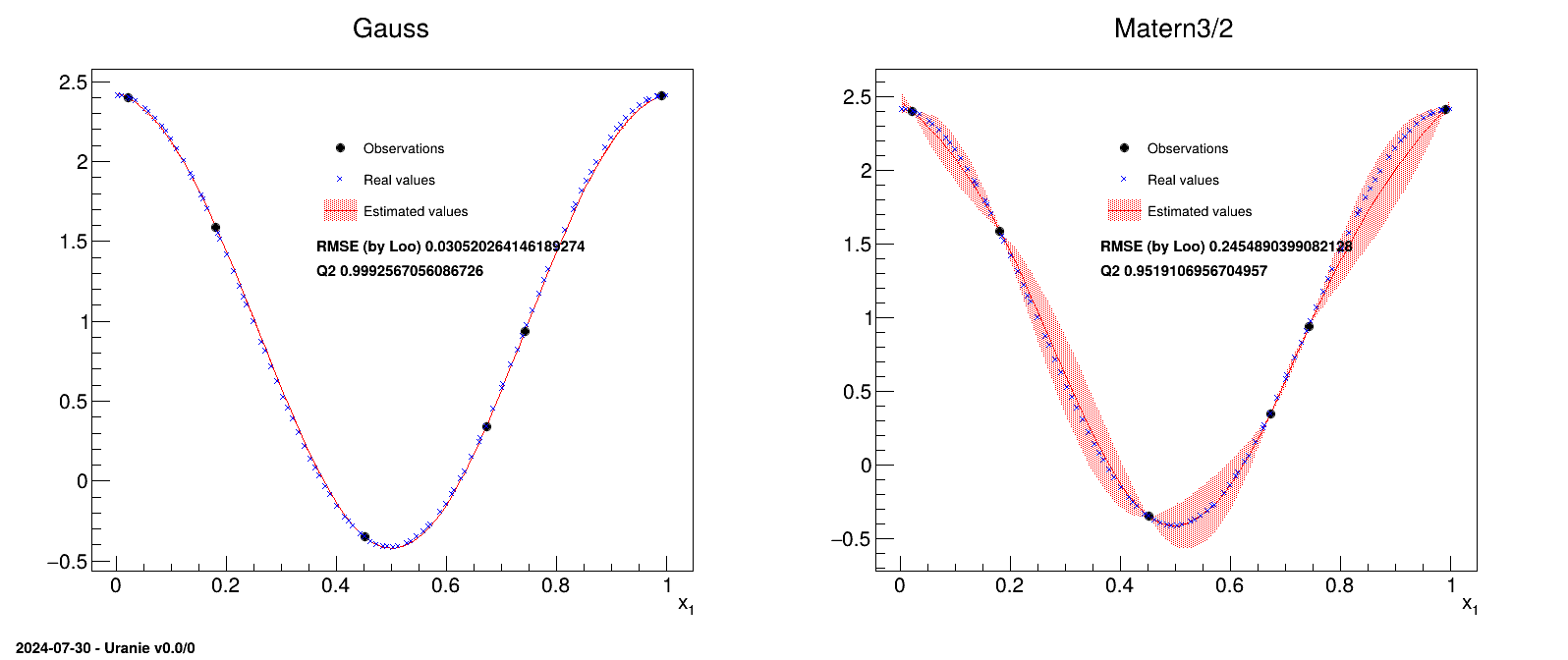
In this example, two different correlation functions are tested and the obtained results are compared at the end.

"""
Example of simple GP usage and illustration of results
"""
from math import sqrt
import numpy as np
from rootlogon import ROOT, DataServer, Modeler, Relauncher


def print_solutions(tds_obs, tds_estim, title):
    """Simple function to produce the 1D plot with observation
    points, testing points along with the uncertainty band."""

    nb_obs = tds_obs.getNPatterns()
    nb_est = tds_estim.getNPatterns()
    rx_arr = np.zeros([nb_est])
    x_arr = np.zeros([nb_est])
    y_est = np.zeros([nb_est])
    y_rea = np.zeros([nb_est])
    std_var = np.zeros([nb_est])

    tds_estim.computeRank("x1")
    tds_estim.getTuple().copyBranchData(rx_arr, nb_est, "Rk_x1")
    tds_estim.getTuple().copyBranchData(x_arr, nb_est, "x1")
    tds_estim.getTuple().copyBranchData(y_est, nb_est, "yEstim")
    tds_estim.getTuple().copyBranchData(y_rea, nb_est, "y")
    tds_estim.getTuple().copyBranchData(std_var, nb_est, "vEstim")

    xarr = np.zeros([nb_est])
    yest = np.zeros([nb_est])
    yrea = np.zeros([nb_est])
    stdvar = np.zeros([nb_est])

    for i in range(nb_est):
        ind = int(rx_arr[i]) - 1
        xarr[ind] = x_arr[i]
        yest[ind] = y_est[i]
        yrea[ind] = y_rea[i]
        stdvar[ind] = 2*sqrt(abs(std_var[i]))

    xobs = np.zeros([nb_obs])
    tds_obs.getTuple().copyBranchData(xobs, nb_obs, "x1")
    yobs = np.zeros([nb_obs])
    tds_obs.getTuple().copyBranchData(yobs, nb_obs, "y")

    gobs = ROOT.TGraph(nb_obs, xobs, yobs)
    gobs.SetMarkerColor(1)
    gobs.SetMarkerSize(1)
    gobs.SetMarkerStyle(8)
    zeros = np.zeros([nb_est])  # use doe plotting only
    gest = ROOT.TGraphErrors(nb_est, xarr, yest, zeros, stdvar)
    gest.SetLineColor(2)
    gest.SetLineWidth(1)
    gest.SetFillColor(2)
    gest.SetFillStyle(3002)
    grea = ROOT.TGraph(nb_est, xarr, yrea)
    grea.SetMarkerColor(4)
    grea.SetMarkerSize(1)
    grea.SetMarkerStyle(5)
    grea.SetTitle("Real Values")

    mgr = ROOT.TMultiGraph("toto", title)
    mgr.Add(gest, "l3")
    mgr.Add(gobs, "P")
    mgr.Add(grea, "P")
    mgr.Draw("A")
    mgr.GetXaxis().SetTitle("x_{1}")

    leg = ROOT.TLegend(0.4, 0.65, 0.65, 0.8)
    leg.AddEntry(gobs, "Observations", "p")
    leg.AddEntry(grea, "Real values", "p")
    leg.AddEntry(gest, "Estimated values", "lf")
    leg.Draw()
    return [mgr, leg]


# Create dataserver and read training database
tdsObs = DataServer.TDataServer("tdsObs", "observations")
tdsObs.fileDataRead("utf-1D-train.dat")
nbObs = 6

# Canvas, divided in 2
Can = ROOT.TCanvas("can", "can", 10, 32, 1600, 700)
apad = ROOT.TPad("apad", "apad", 0, 0.03, 1, 1)
apad.Draw()
apad.Divide(2, 1)

# Name of the plot and correlation functions used
outplot = "GaussAndMatern_1D_AllPoints.png"
Correl = ["Gauss", "Matern3/2"]

# Pointer to needed objects, created in the loop
gpb = [0, 0]
kg = [0, 0]
tdsEstim = [0, 0]
lkrig = [0, 0]

mgs = [0, 0]
legs = [0, 0]
# Looping over the two correlation function chosen
for im in range(2):

    # Create the TGPBuiler object with chosen option to find optimal parameters
    gpb[im] = Modeler.TGPBuilder(tdsObs, "x1", "y", Correl[im], "")
    gpb[im].findOptimalParameters("LOO", 100, "Subplexe", 1000)

    # Get the kriging object
    kg[im] = gpb[im].buildGP()

    # open the dataserver and read the testing basis
    tdsEstim[im] = DataServer.TDataServer("tdsEstim_"+str(im),
                                          "base de test")
    tdsEstim[im].fileDataRead("utf-1D-test.dat")

    # Applied resulting kriging on test basis
    lkrig[im] = Relauncher.TLauncher2(tdsEstim[im], kg[im], "x1",
                                      "yEstim:vEstim")
    lkrig[im].solverLoop()

    # do the plot
    apad.cd(im+1)
    mgs[im], legs[im] = print_solutions(tdsObs, tdsEstim[im], Correl[im])

    lat = ROOT.TLatex()
    lat.SetNDC()
    lat.SetTextSize(0.025)
    lat.DrawLatex(0.4, 0.61, "RMSE (by Loo) "+str(kg[im].getLooRMSE()))
    lat.DrawLatex(0.4, 0.57, "Q2 "+str(kg[im].getLooQ2()))

The first function of this macro (called PrintSolutions) is a complex part that will not be detailed, used to represent the results.

The macro itself starts by reading the training database and storing it in a dataserver. A TGPBuilder is created with the chosen correlation function and the hyper-parameters are estimation by an optimisation procedure in:

gpb[imet] = Modeler.TGPBuilder(tdsObs, "x1", "y", Correl[imet], "");
gpb[imet].findOptimalParameters("LOO", 100, "Subplexe", 1000);

kg[imet] = gpb[imet].buildGP()

The last line shows how to build and retrieve the newly created kriging object.

Finally, this kriging model is tested against the training database, thanks to a TLauncher2 object, as following:

lkrig[imet] = Relauncher.TLauncher2(tdsEstim[imet], kg[imet], "x1", "yEstim:vEstim");
lkrig[imet].solverLoop();