

Documentation
/ Manuel utilisateur en Python
: 
| XIV.12. Macros Calibration | ||
|---|---|---|
 | Chapter XIV. Use-cases in python |  |
This section introduces a few examples of calibration in order to illustrate the different techniques introduced in Chapter XI, along with some of the available options.
The goal here is to calibrate the parameter  within the
 flowrate model, while varying only two inputs
( and
and
 ). The remaining variables
are fixed to the following values:
). The remaining variables
are fixed to the following values:  ,
,  ,
,  ,
,  ,
,  . The context of this example has already been presented in
Section XI.2.4, including the model (implemented here as a C++ function) and the
initial lines defining the
. The context of this example has already been presented in
Section XI.2.4, including the model (implemented here as a C++ function) and the
initial lines defining the TDataServer objects. This macro demonstrates how to apply a simple minimisation approach using
a Relauncher-based architecture.
          """
Example of calibration using minimisation approach on flowrate 1D
"""
from rootlogon import ROOT, DataServer, Relauncher, Reoptimizer, Calibration

# Load the function flowrateCalib1D
ROOT.gROOT.LoadMacro("UserFunctions.C")

# Input reference file
ExpData = "Ex2DoE_n100_sd1.75.dat"

# define the reference
tdsRef = DataServer.TDataServer("tdsRef", "doe_exp_Re_Pr")
tdsRef.fileDataRead(ExpData)

# define the parameters
tdsPar = DataServer.TDataServer("tdsPar", "pouet")
tdsPar.addAttribute(DataServer.TAttribute("hl", 700.0, 760.0))
tdsPar.getAttribute("hl").setDefaultValue(728.0)

# Create the output attribute
out = DataServer.TAttribute("out")

# Create interface to assessors
Model = Relauncher.TCIntEval("flowrateCalib1D")
Model.addInput(tdsPar.getAttribute("hl"))
Model.addInput(tdsRef.getAttribute("rw"))
Model.addInput(tdsRef.getAttribute("l"))
Model.addOutput(out)

# Set the runner
runner = Relauncher.TSequentialRun(Model)

# Set the calibration object
cal = Calibration.TMinimisation(tdsPar, runner, 1)
cal.setDistance("LS", tdsRef, "rw:l", "Qexp")
solv = Reoptimizer.TNloptSubplexe()
cal.setOptimProperties(solv)
cal.estimateParameters()

# Draw the residuals
canRes = ROOT.TCanvas("CanRes", "CanRes", 1200, 800)
padRes = ROOT.TPad("padRes", "padRes", 0, 0.03, 1, 1)
padRes.Draw()
padRes.cd()
cal.drawResiduals("Residuals", "*", "", "nonewcanvas")
Apart from the initial lines described in the section Section XI.2.4, the key step
is to define the starting point of the minimisation. This can be achieved either by calling the
setStartingPoint method of the TNlopt class, or by assigning a
default value to the parameter attributes. In this example, it is done as follows:
tdsPar.getAttribute("hl").setDefaultValue(728.0)
The model is defined (from a TCIntEval instance with the three input variables discussed above,
in the correct order) along with the computation distribution method (sequential).
# Create interface to assessors
Model = Relauncher.TCIntEval("flowrateCalib1D")
Model.addInput(tdsPar.getAttribute("hl"))
Model.addInput(tdsRef.getAttribute("rw"))
Model.addInput(tdsRef.getAttribute("l"))
Model.addOutput(out)

# Set the runner
runner = Relauncher.TSequentialRun(Model)
Once this setup is complete, the calibration object (TMinimisation) is created. As explained in Section XI.2.2.1, the first step is to define the distance function (here the least squares
distance) using setDistance. This method also specifies the TDataServer
containing the reference data, the names of the reference inputs, and the reference variable against which the model
output is compared. Finally, the optimisation algorithm is defined by creating an instance of
TNloptSubplexe, and the parameters are then estimated.
# Set the calibration object
cal = Calibration.TMinimisation(tdsPar,runner,1)
cal.setDistance("LS",tdsRef,"rw:l","Qexp")
solv = Reoptimizer.TNloptSubplexe()
cal.setOptimProperties(solv)
cal.estimateParameters()
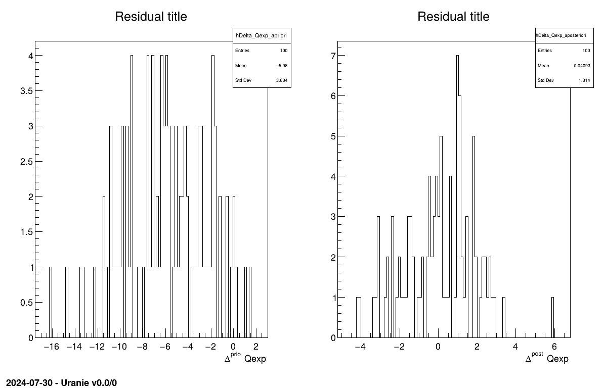
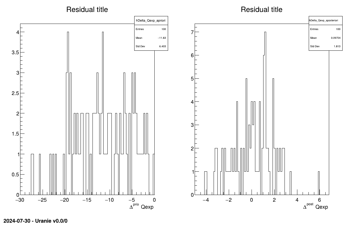
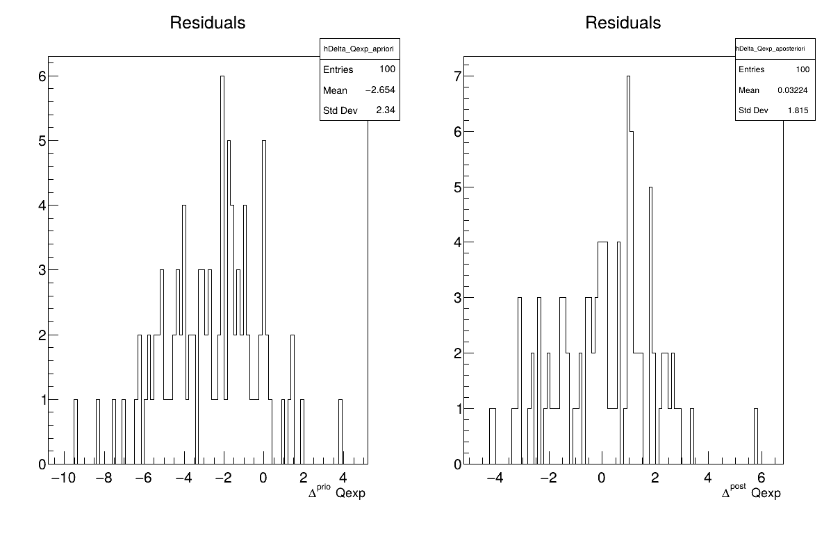
The final part demonstrates how to display the results. Since this method produces a point estimate, only a single value is obtained, which is always shown on the screen, as illustrated in Section XIV.12.1.3. Another important aspect is to examine the residuals, as discussed in [metho]. This is illustrated in Figure XIV.97, which shows the residuals of the a posteriori estimates, typically following a normal distribution.
# Draw the residuals
canRes = ROOT.TCanvas("CanRes", "CanRes", 1200, 800)
padRes = ROOT.TPad("padRes", "padRes", 0, 0.03, 1, 1)
padRes.Draw()
padRes.cd()
cal.drawResiduals("Residuals", "*", "", "nonewcanvas")
          Processing calibrationMinimisationFlowrate1D.py...

--- Uranie v4.11/0 --- Developed with ROOT (6.36.06)
                      Copyright (C) 2013-2026 CEA/DES
                      Contact: support-uranie@cea.fr
                      Date: Tue Feb 10, 2026

|....:....|....:....|....:....|....:
.************************************************
*    Row   * tdsPar__n *     hl.hl * agreement *
************************************************
*        0 *         0 * 749.72363 * 18.149368 *
************************************************
The goal here is to calibrate the parameter parameters  and within the
 flowrateCalib2D model (a two-dimensional version of the
flowrate model), while varying only two inputs
( and
). The remaining variables
are fixed to the following values: , , , , . The context of this example has already been presented in
Section XI.2.4, including the model (implemented here as a C++ function) and the
initial lines defining the TDataServer objects.
In addition to what has been presented in Section XIV.12.1, this macro introduces two new elements:
the use of Vizir instead of a simpler
TNloptSolver-inheriting instance;the discussion of problem identifiability, as introduced in [metho].
          """
Example of calibration through minimisation with Vizir in Flowrate 2D
"""
from rootlogon import ROOT, DataServer, Relauncher, Reoptimizer, Calibration

# Load the function flowrateCalib2DVizir
ROOT.gROOT.LoadMacro("UserFunctions.C")

# Input reference file
ExpData = "Ex2DoE_n100_sd1.75.dat"

# define the reference
tdsRef = DataServer.TDataServer("tdsRef", "doe_exp_Re_Pr")
tdsRef.fileDataRead(ExpData)

# define the parameters
tdsPar = DataServer.TDataServer("tdsPar", "pouet")
tdsPar.addAttribute(DataServer.TAttribute("hu", 1020.0, 1080.0))
tdsPar.addAttribute(DataServer.TAttribute("hl", 720.0, 780.0))

# Create the output attribute
out = DataServer.TAttribute("out")

# Create interface to assessors
Model = Relauncher.TCIntEval("flowrateCalib2D")
Model.addInput(tdsPar.getAttribute("hu"))
Model.addInput(tdsPar.getAttribute("hl"))
Model.addInput(tdsRef.getAttribute("rw"))
Model.addInput(tdsRef.getAttribute("l"))
Model.addOutput(out)

# Set the runner
runner = Relauncher.TSequentialRun(Model)

# Set the calibration object
cal = Calibration.TMinimisation(tdsPar, runner, 1)
cal.setDistance("relativeLS", tdsRef, "rw:l", "Qexp")
# Set optimisaiton properties
solv = Reoptimizer.TVizirGenetic()
solv.setSize(24, 15000, 100)
cal.setOptimProperties(solv)
# cal.getOptimMaster().setTolerance(1e-6)
cal.estimateParameters()

# Draw the residuals
canRes = ROOT.TCanvas("CanRes", "CanRes", 1200, 800)
padRes = ROOT.TPad("padRes", "padRes", 0, 0.03, 1, 1)
padRes.Draw()
padRes.cd()
cal.drawResiduals("Residuals", "*", "", "nonewcanvas")

# Draw the box plot of parameters
canPar = ROOT.TCanvas("CanPar", "CanPar", 1200, 800)
tdsPar.getTuple().SetMarkerStyle(20)
tdsPar.getTuple().SetMarkerSize(0.8)
tdsPar.Draw("hu:hl")

# Look at the correlation and statistic
tdsPar.computeStatistic("hu:hl")
corr = tdsPar.computeCorrelationMatrix("hu:hl")
corr.Print()

print("hl is %3.8g +- %3.8g " % (tdsPar.getAttribute("hl").getMean(),
                                 tdsPar.getAttribute("hl").getStd()))
print("hu is %3.8g +- %3.8g " % (tdsPar.getAttribute("hu").getMean(),
                                 tdsPar.getAttribute("hu").getStd()))
Much of this code has already been covered in the previous section Section XIV.12.1
(up to the sequential run). The main difference here is that the input parameter is now defined as a
TAttribute with boundaries specifying the space in which the algorithm will search.
tdsPar.addAttribute(DataServer.TAttribute("hu", 1020.0, 1080.0) )
tdsPar.addAttribute(DataServer.TAttribute("hl", 720.0, 780.0) )
The model is defined (from a TCIntEval instance with the three input variables discussed above,
in the correct order) along with the computation distribution method (sequential).
# Create interface to assessors
Model = Relauncher.TCIntEval("flowrateCalib2D")
Model.addInput(tdsPar.getAttribute("hu"))
Model.addInput(tdsPar.getAttribute("hl"))
Model.addInput(tdsRef.getAttribute("rw"))
Model.addInput(tdsRef.getAttribute("l"))
Model.addOutput(out)

# Set the runner
runner = Relauncher.TSequentialRun(Model)
Once this setup is complete, the calibration object (TMinimisation) is created. As explained
in Section XI.2.2.1, the first step is to define the distance function (here the
relative least squares distance) using setDistance. This method also specifies the TDataServer
containing the reference data, the names of the reference inputs, and the reference variable against which the model
output is compared. Finally, the optimisation algorithm is defined by creating an instance of
TVizirGenetic, and the parameters are then estimated.
# Set the calibration object
cal = Calibration.TMinimisation(tdsPar,runner,1)
cal.setDistance("relativeLS",tdsRef,"rw:l","Qexp")
# Set optimisation properties
solv = Reoptimizer.TVizirGenetic()
solv.setSize(24,15000,100)
cal.setOptimProperties(solv)
# cal.getOptimMaster().setTolerance(1e-6)
cal.estimateParameters()
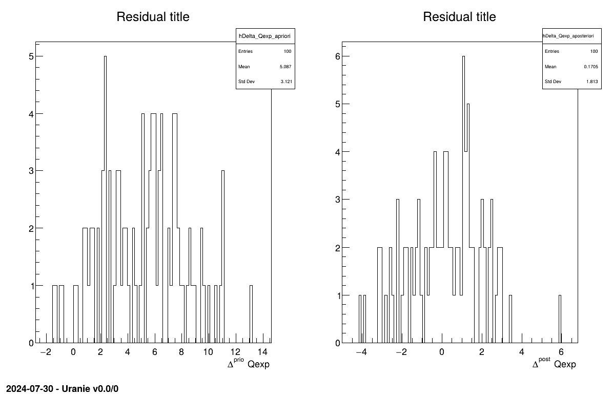
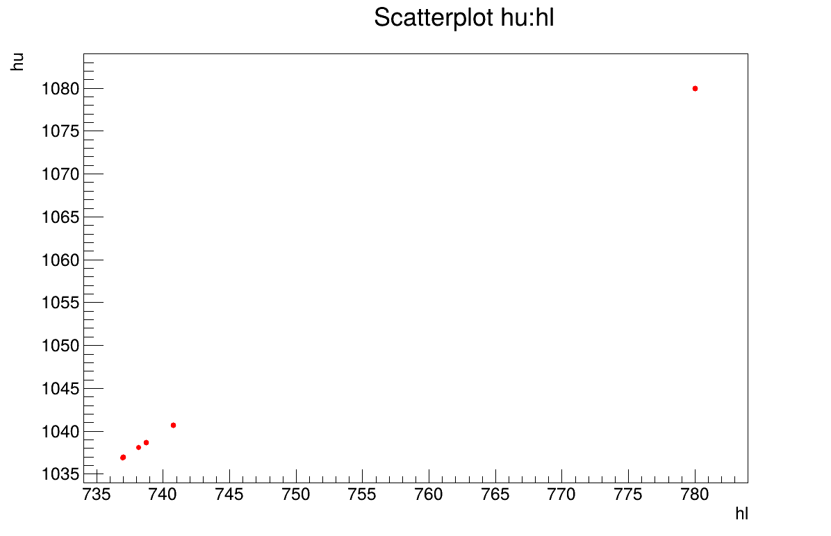
The final part demonstrates how to display the results. Since this method produces a point estimate, only a single value is obtained, which is always shown on the screen, as illustrated in Section XIV.12.2.3. Another important aspect is to examine the residuals, as discussed in [metho]. This is illustrated in Figure XIV.98, which shows the residuals of the a posteriori estimates, typically following a normal distribution. Finally, the parameter graph (Figure XIV.99) reveals a wide variety of possible solutions. This highlights a problem of identifiability, since infinitely many parameter combinations can lead to the same results, as further confirmed by the correlation matrix shown in Section XIV.12.2.3.
# Draw the residuals
canRes = ROOT.TCanvas("CanRes", "CanRes", 1200, 800)
padRes = ROOT.TPad("padRes", "padRes", 0, 0.03, 1, 1)
padRes.Draw()
padRes.cd()
cal.drawResiduals("Residuals", "*", "", "nonewcanvas")

# Draw the box plot of parameters
canPar = ROOT.TCanvas("CanPar", "CanPar", 1200, 800)
tdsPar.getTuple().SetMarkerStyle(20)
tdsPar.getTuple().SetMarkerSize(0.8)
tdsPar.Draw("hu:hl")

# Look at the correlation and statistic
tdsPar.computeStatistic("hu:hl")
corr = tdsPar.computeCorrelationMatrix("hu:hl")
corr.Print()

print("hl is %3.8g +- %3.8g " % (tdsPar.getAttribute("hl").getMean(), tdsPar.getAttribute("hl").getStd()))
print("hu is %3.8g +- %3.8g " % (tdsPar.getAttribute("hu").getMean(), tdsPar.getAttribute("hu").getStd()))
          Processing calibrationMinimisationFlowrate2DVizir.py...

--- Uranie v4.11/0 --- Developed with ROOT (6.36.06)
                      Copyright (C) 2013-2026 CEA/DES
                      Contact: support-uranie@cea.fr
                      Date: Tue Feb 10, 2026

first 100
Genetic  1

  Generation : 1, rang max 23
	Nb d'evaluation : 100, taille de la Z.P. :  0

  Generation : 2, rang max 23
	Nb d'evaluation : 465, taille de la Z.P. :  1

  Generation : 3, rang max 8
	Nb d'evaluation : 963, taille de la Z.P. :  6

  Generation : 4, rang max 0
	Nb d'evaluation : 1617, taille de la Z.P. :  24
Genetic  converge 1617
************************************************************************************
*    Row   * tdsPar__n *     hu.hu *     hl.hl * agreement * rgpareto. * generatio *
************************************************************************************
*        0 *         0 * 1038.1302 * 738.13383 * 0.3639076 *         0 *         3 *
*        1 *         1 *      1080 *       780 * 0.3639083 *         0 *         3 *
*        2 *         2 * 1040.7058 * 740.77116 * 0.3639018 *         0 *         3 *
*        3 *         3 * 1079.9545 *       780 * 0.3639024 *         0 *         3 *
*        4 *         4 * 1040.7058 * 740.77116 * 0.3639018 *         0 *         1 *
*        5 *         5 * 1038.6638 * 738.70819 * 0.3639025 *         0 *         3 *
*        6 *         6 * 1040.7058 * 740.77116 * 0.3639018 *         0 *         3 *
*        7 *         7 * 1036.9776 * 736.98122 * 0.3639076 *         0 *         3 *
*        8 *         8 * 1036.9776 * 736.98122 * 0.3639076 *         0 *         3 *
*        9 *         9 * 1038.6638 * 738.70819 * 0.3639025 *         0 *         3 *
*       10 *        10 * 1036.9776 * 736.98122 * 0.3639076 *         0 *         2 *
*       11 *        11 *      1080 *       780 * 0.3639083 *         0 *         3 *
*       12 *        12 * 1036.9776 * 736.98122 * 0.3639076 *         0 *         3 *
*       13 *        13 * 1040.7058 * 740.77116 * 0.3639018 *         0 *         2 *
*       14 *        14 *      1080 *       780 * 0.3639083 *         0 *         3 *
*       15 *        15 *      1080 *       780 * 0.3639083 *         0 *         3 *
*       16 *        16 * 1038.6638 * 738.70819 * 0.3639025 *         0 *         3 *
*       17 *        17 * 1040.7058 * 740.77116 * 0.3639018 *         0 *         3 *
*       18 *        18 *      1080 *       780 * 0.3639083 *         0 *         3 *
*       19 *        19 * 1036.9776 * 736.98122 * 0.3639076 *         0 *         3 *
*       20 *        20 * 1036.9042 * 736.96108 * 0.3639019 *         0 *         3 *
*       21 *        21 * 1038.6638 * 738.70819 * 0.3639025 *         0 *         3 *
*       22 *        22 *      1080 *       780 * 0.3639083 *         0 *         3 *
*       23 *        23 *      1080 *       780 * 0.3639083 *         0 *         3 *
************************************************************************************

2x2 matrix is as follows

     |      0    |      1    |
-------------------------------
   0 |          1           1
   1 |          1           1

hl is 752.4454 +- 19.946252
hu is 1052.4192 +- 19.959796
The goal here is to calibrate the parameter within the flowrate model, while varying only two inputs
( and
). The remaining variables
are fixed to the following values: , , , , . The context of this example has already been presented in
Section XI.2.4, including the model (implemented here as a C++ function) and the
initial lines defining the TDataServer objects. This macro demonstrates how to apply a linear Bayesian estimation technique
using a Relauncher-based architecture.
          """
Example of linear bayesian calibration with simple 1D flowrate model
"""
from rootlogon import ROOT, DataServer, Relauncher, Calibration

# Load the function flowrateCalib1D
ROOT.gROOT.LoadMacro("UserFunctions.C")

# Input reference file
ExpData = "Ex2DoE_n100_sd1.75.dat"

# define the reference
tdsRef = DataServer.TDataServer("tdsRef", "doe_exp_Re_Pr")
tdsRef.fileDataRead(ExpData)

# define the parameters
tdsPar = DataServer.TDataServer("tdsPar", "pouet")
tdsPar.addAttribute(DataServer.TUniformDistribution("hl", 700.0, 760.0))

# Create the output attribute
out = DataServer.TAttribute("out")

# Create interface to assessors
Reg = Relauncher.TCIntEval("flowrateModelnoH")
Reg.addInput(tdsRef.getAttribute("rw"))
Reg.addInput(tdsRef.getAttribute("l"))
Reg.addOutput(DataServer.TAttribute("H"))
runnoH = Relauncher.TSequentialRun(Reg)
runnoH.startSlave()
if runnoH.onMaster():
    launch = Relauncher.TLauncher2(tdsRef, runnoH)
    launch.solverLoop()
    runnoH.stopSlave()

# Create interface to assessors
Model = Relauncher.TCIntEval("flowrateCalib1D")
Model.addInput(tdsPar.getAttribute("hl"))
Model.addInput(tdsRef.getAttribute("rw"))
Model.addInput(tdsRef.getAttribute("l"))
Model.addOutput(out)

# Set the runner
runner = Relauncher.TSequentialRun(Model)

# Set the covariance matrix of the input reference
sd = tdsRef.getValue("sd_eps", 0)
mat = ROOT.TMatrixD(100, 100)
for ival in range(tdsRef.getNPatterns()):
    mat[ival][ival] = (sd*sd)

# Set the calibration object
cal = Calibration.TLinearBayesian(tdsPar, runner, 1, "")
cal.setLikelihood("gauss_lin", tdsRef, "rw:l", "Qexp")
cal.setObservationCovarianceMatrix(mat)
cal.setRegressorName("H")
cal.setParameterTransformationFunction(ROOT.transf)
cal.estimateParameters()

# Draw the parameters
canPar = ROOT.TCanvas("CanPar", "CanPar", 1200, 800)
padPar = ROOT.TPad("padPar", "padPar", 0, 0.03, 1, 1)
padPar.Draw()
padPar.cd()
cal.drawParameters("Parameters", "*", "nonewcanvas,transformed")

# Draw the residuals
canRes = ROOT.TCanvas("CanRes", "CanRes", 1200, 800)
padRes = ROOT.TPad("padRes", "padRes", 0, 0.03, 1, 1)
padRes.Draw()
padRes.cd()
cal.drawResiduals("Residuals", "*", "", "nonewcanvas")
Much of this code has already been covered in the previous section Section XIV.12.1
(up to the sequential run). The main difference here is that the input parameter is now defined as a
TStochasticDistribution, representing the a priori chosen distribution.
In this example, it can be either a TNormalDistribution or a TUniformDistribution
(see [metho]), with the latter being selected here:
tdsPar.addAttribute(DataServer.TUniformDistribution("hl", 700.0, 760.0) )
Another difference from the previous example is that the method must be slightly adapted to obtain values for the
regressor. As discussed in [metho], linear Bayesian estimation can be applied when the model is approximately linear.
This requires linearising the flowrate function, as demonstrated here:
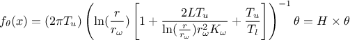
Here, the regressor can be expressed as  .
From this expression, it is clear that we will be calibrating a newly defined parameter
.
From this expression, it is clear that we will be calibrating a newly defined parameter  , which must later be converted back into the parameter of interest. To obtain the regressor
estimation, we simply use another C++ function,
, which must later be converted back into the parameter of interest. To obtain the regressor
estimation, we simply use another C++ function, flowrateModelnoH together with the standard
Relauncher approach:
# Create interface to assessors
Reg = Relauncher.TCIntEval("flowrateModelnoH")
Reg.addInput(tdsRef.getAttribute("rw"))
Reg.addInput(tdsRef.getAttribute("l"))
Reg.addOutput(DataServer.TAttribute("H") )
runnoH = Relauncher.TSequentialRun(Reg)
runnoH.startSlave()
if runnoH.onMaster():
    launch = Relauncher.TLauncher2(tdsRef, runnoH)
    launch.solverLoop()
    runnoH.stopSlave()
This method also requires the input covariance matrix. The provided dataset
(Ex2DoE_n100_sd1.75.dat) contains an estimate of the uncertainty affecting the reference
measurements. Since this uncertainty is constant across all samples, the input covariance matrix is diagonal,
with each diagonal element equal to the square of the standard deviation, as illustrated below:
# Set the covariance matrix of the input reference
sd = tdsRef.getValue("sd_eps",0)
mat = ROOT.TMatrixD(100,100)
for ival in range(tdsRef.getNPatterns()):
    mat[ival][ival] = (sd*sd)
The model is defined (from a TCIntEval instance with the three input variables discussed above,
in the correct order) along with the computation distribution method (sequential).
The calibration object is then created using a Mahalanobis distance function, which is used here for illustrative purposes (see Section XI.4 for more details). The three key steps are:
Providing the input covariance matrix via the
setObservationCovarianceMatrixmethod;Specifying the regressorsâ names using
setRegressorName;Defining the parameter transformation function (optional) with
setParameterTransformationFunction.
The final step is more involved: since we are calibrating  , we need to recover the corresponding parameter value at the end.
This is achieved by providing a C++ function that transforms the parameter estimated from the linearisation back into
the parameter of interest. For illustration, this is implemented in
, we need to recover the corresponding parameter value at the end.
This is achieved by providing a C++ function that transforms the parameter estimated from the linearisation back into
the parameter of interest. For illustration, this is implemented in UserFunctions.C via the
transf function, shown below:
void transf(double *x, double *res)
{
  res[0] = 1050 - x[0]; // simply H_l = \theta - H_u
}
The complete block of code discussed in this section is as follows:
# Set the calibration object
cal = Calibration.TLinearBayesian(tdsPar,runner,1,"")
cal.setLikelihood("gauss_lin", tdsRef, "rw:l", "Qexp")
cal.setObservationCovarianceMatrix(mat)
cal.setRegressorName("H")
cal.setParameterTransformationFunction(ROOT.transf)
cal.estimateParameters()
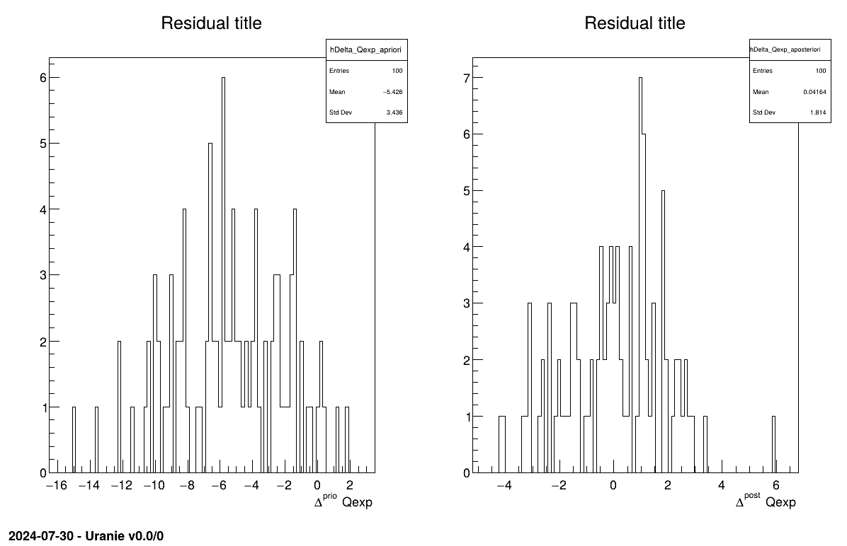
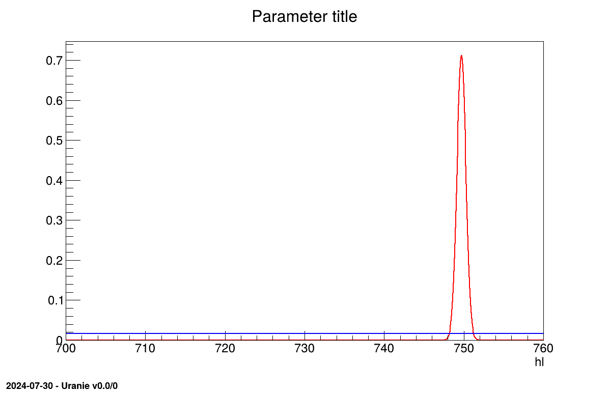
The final part demonstrates how to display the results. Since this method produces normal a posteriori distributions, they are represented by a vector of means and a covariance structure, both easily accessible. The means are displayed on screen, as illustrated in Section XIV.12.3.3. Two additional pieces of a posteriori information are presented as plots: the residuals (Figure XIV.100), which show the expected normal distribution behavior, as discussed in [metho] and the posterior distribution (Figure XIV.101).
# Draw the parameters
canPar = ROOT.TCanvas("CanPar", "CanPar", 1200, 800)
padPar = ROOT.TPad("padPar", "padPar", 0, 0.03, 1, 1)
padPar.Draw()
padPar.cd()
cal.drawParameters("Parameters", "*", "nonewcanvas,transformed")

# Draw the residuals
canRes = ROOT.TCanvas("CanRes", "CanRes", 1200, 800)
padRes = ROOT.TPad("padRes", "padRes", 0, 0.03, 1, 1)
padRes.Draw()
padRes.cd()
cal.drawResiduals("Residuals", "*", "", "nonewcanvas")
          Processing calibrationLinBayesFlowrate1D.py...

--- Uranie v4.11/0 --- Developed with ROOT (6.36.06)
                      Copyright (C) 2013-2026 CEA/DES
                      Contact: support-uranie@cea.fr
                      Date: Tue Feb 10, 2026

***  TLinearBayesian::computeParameters(); Transformed parameters estimated are

1x1 matrix is as follows

     |      0    |
------------------
   0 |      749.7
The goal here is to calibrate the parameter within the flowrate model, while varying only two inputs
( and
). The remaining variables
are fixed to the following values: , , , , . The context of this example has already been presented in
Section XI.2.4, including the model (implemented here as a C++ function) and the
initial lines defining the TDataServer objects. This macro demonstrates how to apply a rejection ABC method
using a Relauncher-based architecture.
          """
Example of calibration using Rejection ABC approach on flowrate 1D
"""
from rootlogon import ROOT, DataServer, Calibration, Relauncher

# Load the function flowrateCalib1D
ROOT.gROOT.LoadMacro("UserFunctions.C")

# Input reference file
ExpData = "Ex2DoE_n100_sd1.75.dat"

# define the reference
tdsRef = DataServer.TDataServer("tdsRef", "doe_exp_Re_Pr")
tdsRef.fileDataRead(ExpData)

# define the parameters
tdsPar = DataServer.TDataServer("tdsPar", "pouet")
tdsPar.addAttribute(DataServer.TUniformDistribution("hl", 700.0, 760.0))

# Create the output attribute
out = DataServer.TAttribute("out")

# Create interface to assessors
Model = Relauncher.TCIntEval("flowrateCalib1D")
Model.addInput(tdsPar.getAttribute("hl"))
Model.addInput(tdsRef.getAttribute("rw"))
Model.addInput(tdsRef.getAttribute("l"))
Model.addOutput(out)

# Set the runner
runner = Relauncher.TSequentialRun(Model)

# Set the calibration object
nABC = 100
eps = 0.05
cal = Calibration.TRejectionABC(tdsPar, runner, nABC, "")
cal.setDistance("LS", tdsRef, "rw:l", "Qexp")
cal.setGaussianNoise("sd_eps")
cal.setPercentile(eps)
cal.estimateParameters()

# Draw the parameters
canPar = ROOT.TCanvas("CanPar", "CanPar", 1200, 800)
padPar = ROOT.TPad("padPar", "padPar", 0, 0.03, 1, 1)
padPar.Draw()
padPar.cd()
cal.drawParameters("Parameters", "*", "nonewcanvas")

# Draw the residuals
canRes = ROOT.TCanvas("CanRes", "CanRes", 1200, 800)
padRes = ROOT.TPad("padRes", "padRes", 0, 0.03, 1, 1)
padRes.Draw()
padRes.cd()
cal.drawResiduals("Residuals", "*", "", "nonewcanvas")


# Compute statistics
tdsPar.computeStatistic()
print("The mean of hl is %3.8g" % (tdsPar.getAttribute("hl").getMean()))
print("The std of hl is %3.8g" % (tdsPar.getAttribute("hl").getStd()))
Much of this code has already been covered in the previous section Section XIV.12.1
(up to the sequential run). The main difference here is that the input parameter is now defined as a
TStochasticDistribution, representing the a priori chosen distribution.
tdsPar.addAttribute(DataServer.TUniformDistribution("hl", 700.0, 760.0) )
The model is defined (from a TCIntEval instance with the three input variables discussed above,
in the correct order) along with the computation distribution method (sequential).
The calibration object is then created by specifying both the number of elements in the final sample
(nABC = 100) and the percentile of events retained (eps = 0.05, meaning that 2000
locations will be tested). Since the code is deterministic, uncertainty is introduced by adding random Gaussian
noise. The standard deviation of this noise is defined on an event-by-event basis using a variable from the
observation dataserver. Finally, the distance function is specified, and the estimation process is performed.
# Set the calibration object
nABC = 100
eps = 0.05
cal = Calibration.TRejectionABC(tdsPar, runner, nABC, "")
cal.setDistance("LS",tdsRef,"rw:l","Qexp")
cal.setGaussianNoise("sd_eps")
cal.setPercentile(eps)
cal.estimateParameters()
The final part demonstrates how to display the results. Since this method produces samples of the a posteriori distributions, basic statistical information are directly displayed on screen, as shown in Section XIV.12.4.3. Two additional pieces of a posteriori information are presented as plots: the residuals (Figure XIV.102), which show the expected normal distribution behavior, as discussed in [metho] and the posterior distribution (Figure XIV.103).
# Draw the parameters
canPar = ROOT.TCanvas("CanPar", "CanPar", 1200, 800)
padPar = ROOT.TPad("padPar", "padPar", 0, 0.03, 1, 1)
padPar.Draw()
padPar.cd()
cal.drawParameters("Parameters", "*", "nonewcanvas")

# Draw the residuals
canRes = ROOT.TCanvas("CanRes", "CanRes", 1200, 800)
padRes = ROOT.TPad("padRes", "padRes", 0, 0.03, 1, 1)
padRes.Draw()
padRes.cd()
cal.drawResiduals("Residuals", "*", "", "nonewcanvas")

# Compute statistics
tdsPar.computeStatistic()
print("The mean of hl is %3.8g" % (tdsPar.getAttribute("hl").getMean()))
print("The std of hl is %3.8g" % (tdsPar.getAttribute("hl").getStd()))
          Processing calibrationRejectionABCFlowrate1D.py...

--- Uranie v4.11/0 --- Developed with ROOT (6.36.06)
                      Copyright (C) 2013-2026 CEA/DES
                      Contact: support-uranie@cea.fr
                      Date: Tue Feb 10, 2026

 <URANIE::INFO>
 <URANIE::INFO> *** URANIE INFORMATION ***
 <URANIE::INFO> *** File[${SOURCEDIR}/meTIER/calibration/souRCE/TDistanceLikelihoodFunction.cxx] Line[601]
 <URANIE::INFO> TDistanceLikelihoodFunction::setGaussianRandomNoise: gaussian random noise(s) is added using information in [sd_eps] to modify the output variable(s) [out].
 <URANIE::INFO> *** END of URANIE INFORMATION ***
 <URANIE::INFO>
 <URANIE::INFO>
 <URANIE::INFO> *** URANIE INFORMATION ***
 <URANIE::INFO> *** File[${SOURCEDIR}/meTIER/calibration/souRCE/TRejectionABC.cxx] Line[118]
 <URANIE::INFO> TRejectionABC::computeParameters:: 2000 evaluations will be performed !
 <URANIE::INFO> *** END of URANIE INFORMATION ***
 <URANIE::INFO>
A posteriori mean coordinates are : (749.926)
The mean of hl is 749.92609
The std of hl is 1.9704229
The goal here is to calibrate the parameter within the flowrate model, while varying only two inputs
( and
). The remaining variables
are fixed to the following values: , , , , . The context of this example has already been presented in
Section XI.2.4, including the model (implemented here as a C++ function) and the
initial lines defining the TDataServer objects. This macro demonstrates how to apply the Markov chain Monte Carlo
approach and more precisely the component-wise Metropolis-Hastings algorithm using a
Relauncher-based architecture.
"""
Example of MCMC usage on simple flowrate 1D model
"""
from rootlogon import ROOT, DataServer, Relauncher, Calibration

# Load the function flowrateCalib1D
ROOT.gROOT.LoadMacro("UserFunctions.C")

# Input reference file
ExpData = "Ex2DoE_n100_sd1.75.dat"

# Define the reference
tdsRef = DataServer.TDataServer("tdsRef", "doe_exp_Re_Pr")
tdsRef.fileDataRead(ExpData)

# Define the parameters
tdsPar = DataServer.TDataServer("tdsPar", "pouet")
tdsPar.addAttribute(DataServer.TUniformDistribution("hl", 700.0, 760.0))

# Create the output attribute
out = DataServer.TAttribute("out")

# Create interface to assessors
Model = Relauncher.TCIntEval("flowrateCalib1D")
Model.addInput(tdsPar.getAttribute("hl"))
Model.addInput(tdsRef.getAttribute("rw"))
Model.addInput(tdsRef.getAttribute("l"))
Model.addOutput(out)

# Set the runner
runner = Relauncher.TSequentialRun(Model)

# Set the calibration object
cal = Calibration.TMCMC(tdsPar, runner, 2000)

# Set the likelihood and reference with default gaussian log likelihood
cal.setLikelihood("log-gauss",tdsRef,"rw:l","Qexp","sd_eps")

# Set the MCMC algorithm to component-wise Metropolis-Hastings
cal.setAlgo("MH_1D")

# Set the acceptation ratio range between 20% and 50%
cal.setAcceptationRatioRange(0.2, 0.5)

# Set the number of iterations between two information displays
cal.setNbDump(500)

# Initialise 4 chains
cal.setMultistart(4)


# Set the starting points of each chain
cal.setStartingPoints(0, [740])
cal.setStartingPoints(1, [745])
cal.setStartingPoints(2, [750])
cal.setStartingPoints(3, [755])

# Set the standard deviation of the proposal for all the chains
cal.setProposalStd(-1, [5])

# Run the MCMC algorithm
cal.estimateParameters()

# Quality assessment: Draw the trace of the Markov Chain
canTr = ROOT.TCanvas("CanTr","CanTr",1200,800)
padTr = ROOT.TPad("padTr","padTr",0, 0.03, 1, 1)
padTr.Draw()
padTr.cd()
cal.drawTrace("Trace", "*", "nonewcanvas")

# Quality assessment: Draw the acceptation ratio
canAcc = ROOT.TCanvas("CanAcc","CanAcc",1200,800)
padAcc = ROOT.TPad("padAcc","padAcc",0, 0.03, 1, 1)
padAcc.Draw()
padAcc.cd()
cal.drawAcceptationRatio("Acceptation ratio", "*", "nonewcanvas")

# Set the number of iterations to remove
burnin = 50
cal.setBurnin(burnin)

# Verify that the burn-in has been set correctely with Gelman-Rubin statistic
GelmanRubin_values = cal.diagGelmanRubin()

# Compute Effective Sample Size
ESS_values = cal.diagESS()

# Set the lag
lag = 1
cal.setLag(lag)

# Draw the residuals
canRes = ROOT.TCanvas("CanRes","CanRes",1200,800);
padRes = ROOT.TPad("padRes","padRes",0, 0.03, 1, 1)
padRes.Draw()
padRes.cd()
cal.drawResiduals("Residuals", "*", "", "nonewcanvas")

# Draw the posterior distributions
canPar = ROOT.TCanvas("CanPar","CanPar",1200,800)
padPar = ROOT.TPad("padPar","padPar",0, 0.03, 1, 1)
padPar.Draw()
padPar.cd()
cal.drawParameters("Posterior", "*", "nonewcanvas")
Much of this code has already been covered in the previous section Section XIV.12.1
(up to the sequential run). The main difference here is that the input parameter is now defined as a
TStochasticDistribution, representing the a priori chosen distribution.
tdsPar.addAttribute(DataServer.TUniformDistribution("hl", 700.0, 760.0) )
The model is defined (from a TCIntEval instance with the three input variables discussed above,
in the correct order) along with the computation distribution method (sequential).
The calibration object is then created by specifying both the number of iterations of the algorithm (set to 2000). The likelihood function is defined as Gaussian, with the reference dataserver, the input and output variables, and the standard deviation of the experimental data provided as arguments. Several additional options are configured: the component-wise algorithm is selected, the acceptance range is set, the interval between two console displays is specified, the number of chains to initialise is defined, the starting points of each chain are assigned (one by one), and the standard deviation of the initial proposal distribution is set (for all chains at once). For further details on these options, see Section XI.6.2. Finally, the estimation process is performed, using the chosen MCMC algorithm (component-wise Metropolis-Hastings).
# Set the calibration object
cal = Calibration.TMCMC(tdsPar, runner, 2000)

# Set the likelihood and reference with default gaussian log likelihood
cal.setLikelihood("log-gauss",tdsRef,"rw:l","Qexp","sd_eps")

# Set the MCMC algorithm to component-wise Metropolis-Hastings
cal.setAlgo("MH_1D")

# Set the acceptation ratio range between 20% and 50%
cal.setAcceptationRatioRange(0.2, 0.5)

# Set the number of iterations between two information displays
cal.setNbDump(500)

# Initialise 4 chains
cal.setMultistart(4)

# Set the starting points of each chain
cal.setStartingPoints(0, [740])
cal.setStartingPoints(1, [745])
cal.setStartingPoints(2, [750])
cal.setStartingPoints(3, [755])

# Set the standard deviation of the proposal for all the chains
cal.setProposalStd(-1, [5])

# Run the MCMC algorithm
cal.estimateParameters()
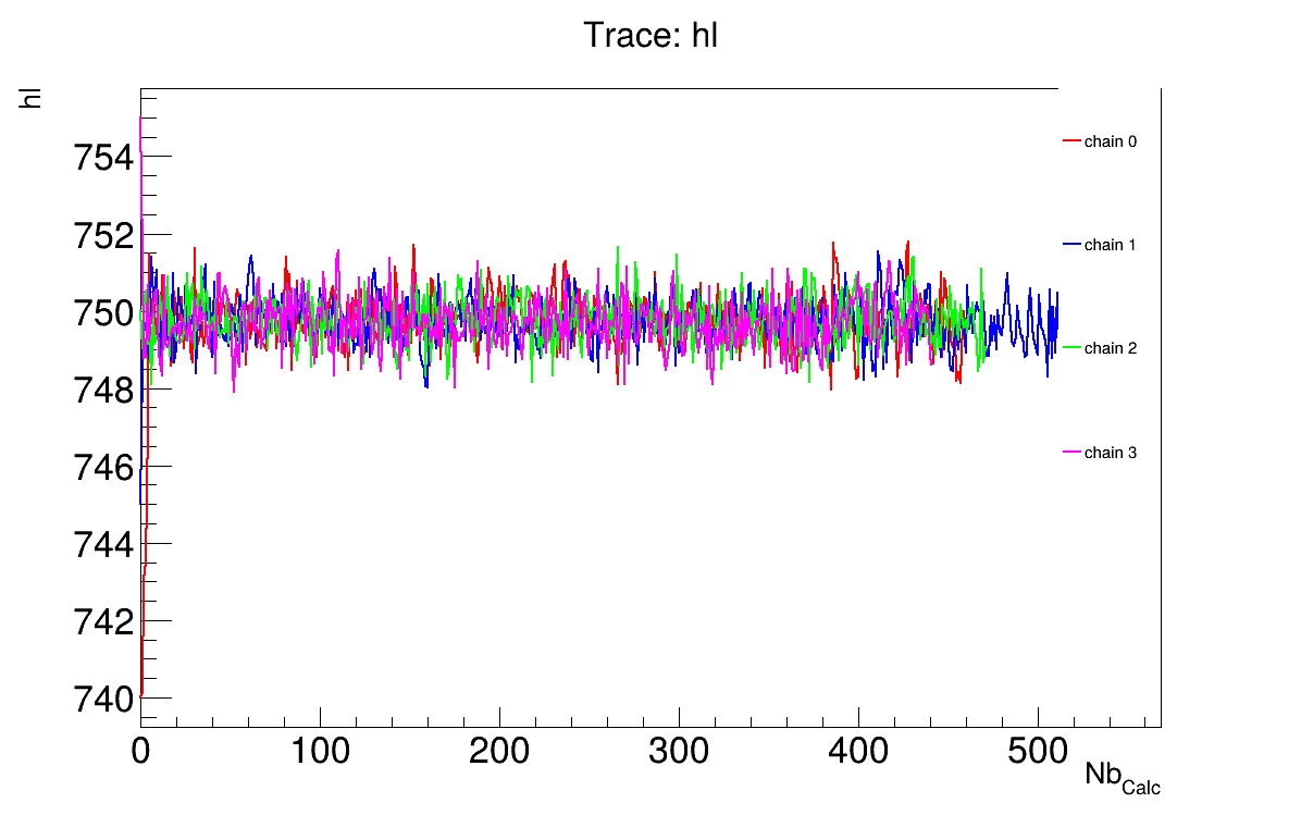
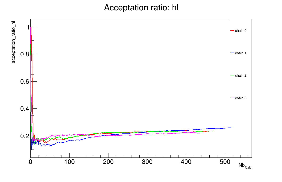
The final part demonstrates how to display and analyse the results. The first elements to examine are the trace plot (Figure XIV.104) and the acceptance ratio plot (Figure XIV.105). On these plots, you should check that the number of accepted iterations is sufficiently high (at least several hundred if the chains stabilise quickly, in our case, around 500), and that the converged acceptance ratio falls within a reasonable range (20-50%, here, it is close to 25%). When inspecting the trace, the chains should have converged around the same region (as they do here), and they should evolve rapidly, which indicates efficient exploration and low autocorrelation (also observed in our case). Finally, these plots help verify whether all chains behave stably and from which iteration they can be considered stable. This provides a first indication of a suitable burn-in value. In this example, the chains appear to have converged, and a burn-in value of 50 seems appropriate.
The burn-in size can then be defined and its consistency verified using the Gelman-Rubin statistic. In our case, a value of 1.00137 is reported in Section XIV.12.5.3 which is very close to 1 and confirms excellent convergence of the chains. Otherwise, a different burn-in value might have been more appropriate, the calculation could have been extended, or the MCMC algorithm settings adjusted.
The next step is to check for sample autocorrelation within the chains. The Effective Sample Size (ESS) provides a good indication of the lag to be used. In our case, the chains contain a reasonable number of independent samples (at least 257 each), and a lag of 1 is sufficient (see Section XIV.12.5.3). Otherwise, the calculation could have been extended, or the MCMC algorithm settings adjusted (especially the standard deviation of the proposal distribution).
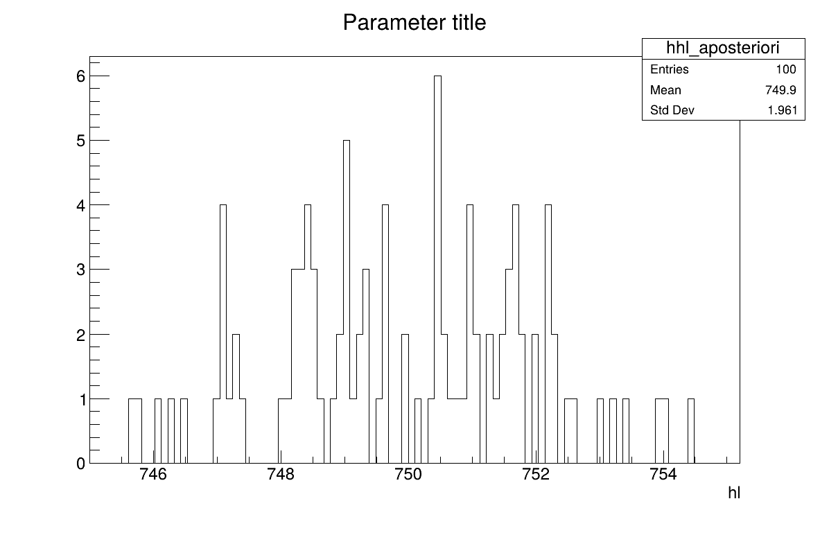
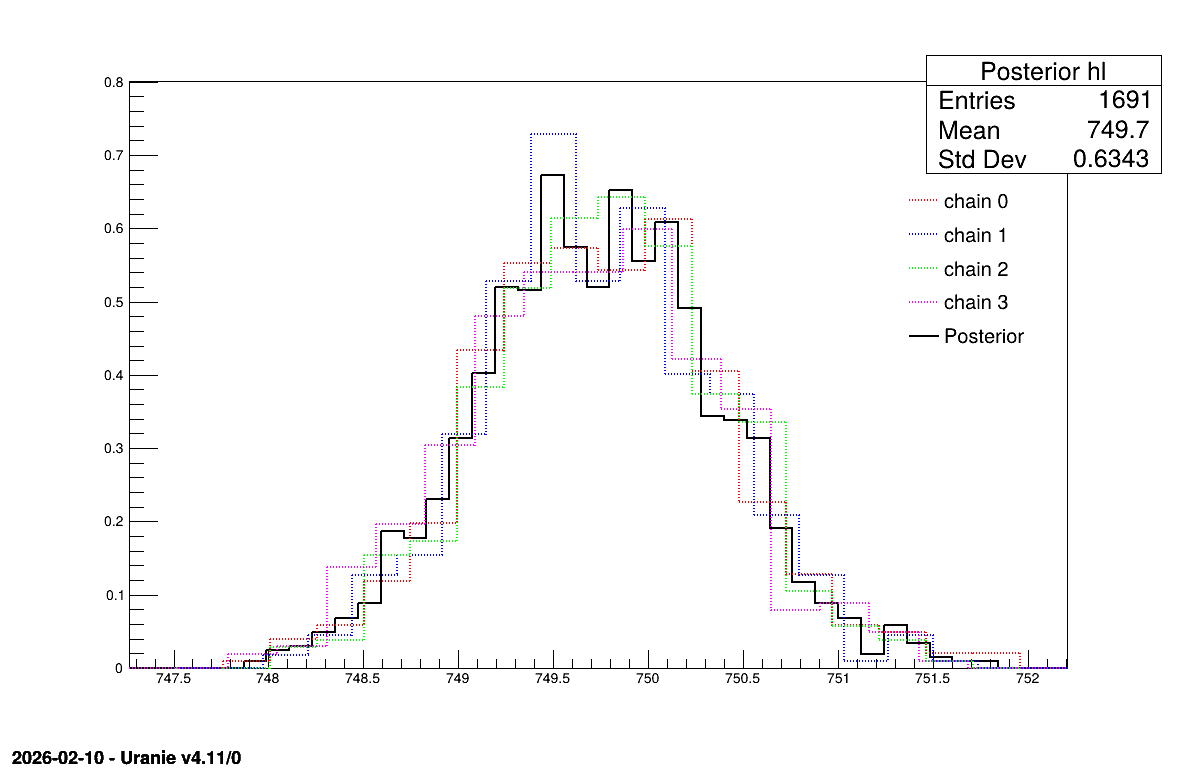
Two additional pieces of a posteriori information are presented as plots: the residuals (Figure XIV.106), which show the expected normal distribution behavior, as discussed in [metho] and the posterior distribution (Figure XIV.107).
# Quality assessment: Draw the trace of the Markov Chain
canTr = ROOT.TCanvas("CanTr","CanTr",1200,800)
padTr = ROOT.TPad("padTr","padTr",0, 0.03, 1, 1)
padTr.Draw()
padTr.cd()
cal.drawTrace("Trace", "*", "nonewcanvas")

# Quality assessment: Draw the acceptation ratio
canAcc = ROOT.TCanvas("CanAcc","CanAcc",1200,800)
padAcc = ROOT.TPad("padAcc","padAcc",0, 0.03, 1, 1)
padAcc.Draw()
padAcc.cd()
cal.drawAcceptationRatio("Acceptation ratio", "*", "nonewcanvas")

# Set the number of iterations to remove
burnin = 50
cal.setBurnin(burnin)

# Verify that the burn-in has been set correctely with Gelman-Rubin statistic
GelmanRubin_values = cal.diagGelmanRubin()

# Compute Effective Sample Size
ESS_values = cal.diagESS()

# Set the lag
lag = 1
cal.setLag(lag)

# Draw the residuals
canRes = ROOT.TCanvas("CanRes", "CanRes", 1200, 800)
padRes = ROOT.TPad("padRes", "padRes", 0, 0.03, 1, 1)
padRes.Draw()
padRes.cd()
cal.drawResiduals("Residuals", "*", "", "nonewcanvas")

# Draw the posterior distributions
canPar = ROOT.TCanvas("CanPar", "CanPar", 1200, 800)
padPar = ROOT.TPad("padPar", "padPar", 0, 0.03, 1, 1)
padPar.Draw()
padPar.cd()
cal.drawParameters("Posterior", "*", "nonewcanvas")
          Processing calibrationMCMCFlowrate1D.py...

--- Uranie v4.11/0 --- Developed with ROOT (6.36.06)
                      Copyright (C) 2013-2026 CEA/DES
                      Contact: support-uranie@cea.fr
                      Date: Tue Feb 10, 2026

 <URANIE::INFO>
 <URANIE::INFO> *** URANIE INFORMATION ***
 <URANIE::INFO> *** File[${SOURCEDIR}/meTIER/calibration/souRCE/TMCMC.cxx] Line[193]
 <URANIE::INFO> TMCMC::constructor
 <URANIE::INFO> A folder named [MCMC_1] has been created to store the results of the new calculation.
 <URANIE::INFO> *** END of URANIE INFORMATION ***
 <URANIE::INFO>

 <URANIE::INFO>
 <URANIE::INFO> *** URANIE INFORMATION ***
 <URANIE::INFO> *** File[${SOURCEDIR}/meTIER/calibration/souRCE/TMCMC.cxx] Line[673]
 <URANIE::INFO> TMCMC::constructor
 <URANIE::INFO> MCMC_1_chain_0 file has been duplicated in the folder [MCMC_1] to initiate [4] chains.
 <URANIE::INFO> *** END of URANIE INFORMATION ***
 <URANIE::INFO>

500 events done
1000 events done
1500 events done
2000 events done
Computation finished with 2000 iterations.
Acceptation ratio [22.95%].
A posteriori mean coordinates are : (749.692)
500 events done
1000 events done
1500 events done
2000 events done
Computation finished with 2000 iterations.
Acceptation ratio [25.8%].
A posteriori mean coordinates are : (749.727)
500 events done
1000 events done
1500 events done
2000 events done
Computation finished with 2000 iterations.
Acceptation ratio [23.55%].
A posteriori mean coordinates are : (749.769)
500 events done
1000 events done
1500 events done
2000 events done
Computation finished with 2000 iterations.
Acceptation ratio [22.05%].
A posteriori mean coordinates are : (749.713)

Gelman-Rubin statistic for variable [hl] is equal to 1.00137. Excellent convergence.

Effective Sample Size (ESS) for variable [hl] and chain [0] is equal to 257.
Effective Sample Size (ESS) for variable [hl] and chain [1] is equal to 305.
Effective Sample Size (ESS) for variable [hl] and chain [2] is equal to 405.
Effective Sample Size (ESS) for variable [hl] and chain [3] is equal to 371.

For uncorrelated samples, the lag should be set to 1.
The goal here is to calibrate the parameters  (constant term) and
  (multiplicative term) within a simple linear model (implemented in
 UserFunctions.C), against the
observable outputs  , associated
with given values of
, associated
with given values of  stored in
the input file
stored in
the input file linReg_Database.dat. The initial lines defining the TDataServer and the model are similar
to those presented in Section XI.2.4. This macro demonstrates how to apply the Markov chain Monte Carlo
approach and more precisely the classic Metropolis-Hastings algorithm in two dimensions using a
Relauncher-based architecture.
"""
Example of calibration using MCMC algo on linear model
"""
from rootlogon import ROOT, DataServer, Relauncher, Calibration
# Load the function Toy
ROOT.gROOT.LoadMacro("UserFunctions.C")
# Input reference file
ExpData = "linReg_Database.dat"
# Define the reference
tdsRef = DataServer.TDataServer("tdsRef", "doe_exp_Re_Pr")
tdsRef.fileDataRead(ExpData)
# Define the uncertainty model guessing the standard deviation (here 0.2)
tdsRef.addAttribute("sd_eps", "0.2")
# Define the parameters
tdsPar = DataServer.TDataServer("tdsPar", "tdsPar")
binf_sea = -2.0
bsup_sea = 2.0
tdsPar.addAttribute(DataServer.TUniformDistribution("t0", binf_sea, bsup_sea))
tdsPar.addAttribute(DataServer.TUniformDistribution("t1", binf_sea, bsup_sea))
# Create the output attribute
out = DataServer.TAttribute("out")
# Create interface to assessors
myeval = Relauncher.TCIntEval("Toy")
myeval.addInput(tdsRef.getAttribute("x"))
myeval.addInput(tdsPar.getAttribute("t0"))
myeval.addInput(tdsPar.getAttribute("t1"))
myeval.addOutput(out)
# Set the runner
run = Relauncher.TSequentialRun(myeval)
# Set the calibration object with default Metropolis-Hastings algorithm
cal = Calibration.TMCMC(tdsPar, run, 4000)
# Set the likelihood and reference with default gaussian log likelihood
cal.setLikelihood("log-gauss", tdsRef, "x", "yExp", "sd_eps")
# Set the number of iterations between two information displays
cal.setNbDump(1000)
# Initialise 4 chains
cal.setMultistart(4)
# Set the starting points of each chain
cal.setStartingPoints(0, [0.5, -0.2])
cal.setStartingPoints(1, [-1.5, 1])
cal.setStartingPoints(2, [-1.2, -0.2])
cal.setStartingPoints(3, [0.3, 0.8])
# Set the standard deviation of the proposal for all the chains
cal.setProposalStd(-1, [0.05, 0.05])
# Run the MCMC algorithm
cal.estimateParameters()
# Quality assessment: Draw the trace of the Markov Chain
canTr = ROOT.TCanvas("CanTr", "CanTr", 1200, 800)
padTr = ROOT.TPad("padTr", "padTr", 0, 0.03, 1, 1)
padTr.Draw()
padTr.cd()
cal.drawTrace("Trace", "*", "nonewcanvas")
# Quality assessment: Draw the acceptation ratio
canAcc = ROOT.TCanvas("CanAcc", "CanAcc", 1200, 800)
padAcc = ROOT.TPad("padAcc", "padAcc", 0, 0.03, 1, 1)
padAcc.Draw()
padAcc.cd()
cal.drawAcceptationRatio("Acceptation ratio", "*", "nonewcanvas")
# Set the number of iterations to remove
burnin = 100
cal.setBurnin(burnin)
# Verify that the burn-in has been set correctely with Gelman-Rubin statistic
GelmanRubin_values = cal.diagGelmanRubin()
# Compute Effective Sample Size
ESS_values = cal.diagESS()
# Set the lag
lag = 3
cal.setLag(lag)
# Quality assessment: Draw the 2D trace of the Markov Chain
canTr2D = ROOT.TCanvas("CanTr2D", "CanTr2D", 1200, 800)
padTr2D = ROOT.TPad("padTr2D", "padTr2D", 0, 0.03, 1, 1)
padTr2D.Draw()
padTr2D.cd()
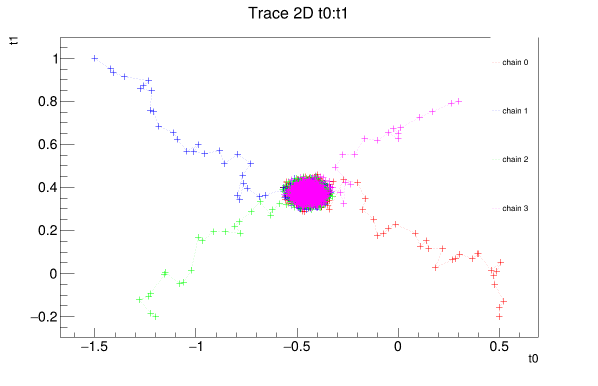
cal.draw2DTrace("Trace 2D", "t0:t1", "nonewcanvas")
# Draw the residuals
canRes = ROOT.TCanvas("CanRes","CanRes",1200,800);
padRes = ROOT.TPad("padRes","padRes",0, 0.03, 1, 1)
padRes.Draw()
padRes.cd()
cal.drawResiduals("Residuals", "*", "", "nonewcanvas")
# Draw the posterior distributions
canPar = ROOT.TCanvas("CanPar","CanPar",1200,800)
padPar = ROOT.TPad("padPar","padPar",0, 0.03, 1, 1)
padPar.Draw()
padPar.cd()
cal.drawParameters("Posterior", "*", "nonewcanvas")
Much of this code has already been covered in the previous section Section XIV.12.1
(up to the sequential run). The main difference here is that the input parameter is now defined as a
TStochasticDistribution, representing the a priori chosen distribution.
Another difference from the previous example Section XIV.12.5 is that no uncertainty
associated with the observables is provided in the input file. To this end, a new attribute is defined and added to the
reference dataserver, with an assumed standard deviation of equal to 0.2.
# Define the uncertainty model guessing the standard deviation (here 0.2)
tdsRef.addAttribute("sd_eps", "0.2")

# Define the parameters
tdsPar = DataServer.TDataServer("tdsPar", "tdsPar")
binf_sea = -2.0
bsup_sea = 2.0
tdsPar.addAttribute(DataServer.TUniformDistribution("t0", binf_sea, bsup_sea))
tdsPar.addAttribute(DataServer.TUniformDistribution("t1", binf_sea, bsup_sea))
The model is defined (from a TCIntEval instance with the three input variables discussed above,
in the correct order) along with the computation distribution method (sequential).
The calibration object is then created by specifying both the number of iterations of the algorithm (set to 4000). The likelihood function is defined as Gaussian, with the reference dataserver, the input and output variables, and the assumed standard deviation of the experimental data (see previous paragraph) provided as arguments. Several additional options are configured: the interval between two console displays is specified, the number of chains to initialise is defined, the starting points of each chain are assigned (one by one), and the standard deviation of the initial proposal distribution is set (for all chains at once). For further details on these options, see Section XI.6.2. Finally, the estimation process is performed, using the default MCMC algorithm (classic Metropolis-Hastings).
# Set the calibration object with default Metropolis-Hastings algorithm
cal = Calibration.TMCMC(tdsPar, run, 4000)

# Set the likelihood and reference with default gaussian log likelihood
cal.setLikelihood("log-gauss", tdsRef, "x", "yExp", "sd_eps")

# Set the number of iterations between two information displays
cal.setNbDump(1000)

# Initialise 4 chains
cal.setMultistart(4)

# Set the starting points of each chain
cal.setStartingPoints(0, [0.5, -0.2])
cal.setStartingPoints(1, [-1.5, 1])
cal.setStartingPoints(2, [-1.2, -0.2])
cal.setStartingPoints(3, [0.3, 0.8])

# Set the standard deviation of the proposal for all the chains
cal.setProposalStd(-1, [0.05, 0.05])

# Run the MCMC algorithm
cal.estimateParameters()
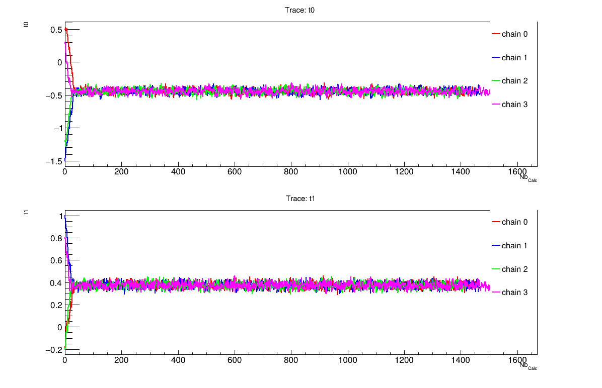
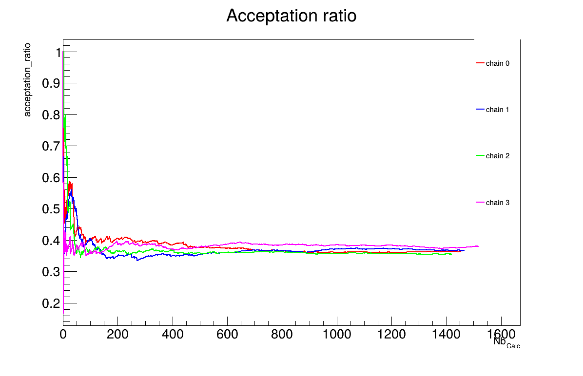
The final part demonstrates how to display and analyse the results. The first elements to examine are the trace plot (Figure XIV.108) and the acceptance ratio plot (Figure XIV.109). On these plots, you should check that the number of accepted iterations is sufficiently high (at least several hundred if the chains stabilise quickly, in our case, around 1500), and that the converged acceptance ratio falls within a reasonable range (20â50%, here, it is close to 40%). When inspecting the trace, the chains should have converged around the same region (as they do here), and they should evolve rapidly, which indicates efficient exploration and low autocorrelation (also observed in our case). Finally, these plots help verify whether all chains behave stably and from which iteration they can be considered stable. This provides a first indication of a suitable burn-in value. In this example, the chains appear to have converged, and a burn-in value of 100 seems appropriate.
The burn-in size can then be defined and its consistency verified using the Gelman-Rubin statistic. In our case,
values of 1.00092 and 0.99993 (for parameters and respectively)
are reported in Section XIV.12.6.3 which are very close to 1 and confirms
excellent convergence of the chains for both parameters. Otherwise, a different burn-in value might have been more
appropriate, the calculation could have been extended, or the MCMC algorithm settings adjusted.
The next step is to check for sample autocorrelation within the chains. The Effective Sample Size (ESS) provides a good indication of the lag to be used. In our case, the chains contain a reasonable number of independent samples (at least 424 each), and a lag of 3 is sufficient (see Section XIV.12.6.3). Otherwise, the calculation could have been extended, or the MCMC algorithm settings adjusted (especially the standard deviation of the proposal distribution).
It is also possible to represent the chains in two dimensions (Figure XIV.110). This provides an alternative way to verify whether the chains converge to the same region and highlights potential covariance between the posterior distributions of the two parameters.
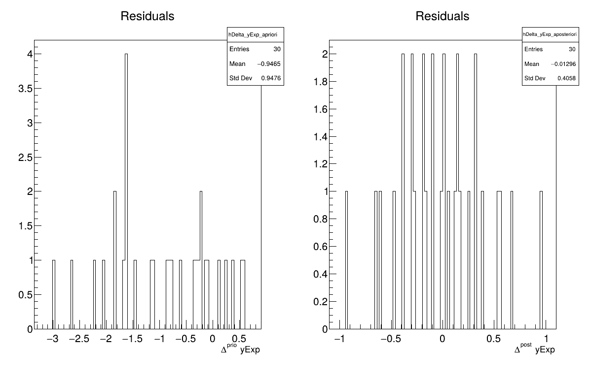
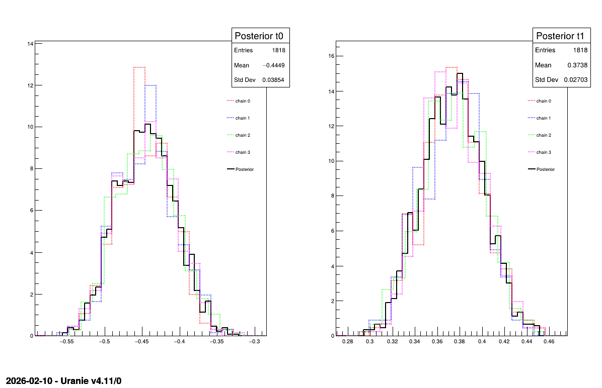
Two additional pieces of a posteriori information are presented as plots: the residuals (Figure XIV.111), which show the expected normal distribution behavior, as discussed in [metho] and the posterior distribution (Figure XIV.112).
# Quality assessment: Draw the trace of the Markov Chain
canTr = ROOT.TCanvas("CanTr", "CanTr", 1200, 800)
padTr = ROOT.TPad("padTr", "padTr", 0, 0.03, 1, 1)
padTr.Draw()
padTr.cd()
cal.drawTrace("Trace", "*", "nonewcanvas")

# Quality assessment: Draw the acceptation ratio
canAcc = ROOT.TCanvas("CanAcc", "CanAcc", 1200, 800)
padAcc = ROOT.TPad("padAcc", "padAcc", 0, 0.03, 1, 1)
padAcc.Draw()
padAcc.cd()
cal.drawAcceptationRatio("Acceptation ratio", "*", "nonewcanvas")

# Set the number of iterations to remove
burnin = 100
cal.setBurnin(burnin)

# Verify that the burn-in has been set correctely with Gelman-Rubin statistic
GelmanRubin_values = cal.diagGelmanRubin()

# Compute Effective Sample Size
ESS_values = cal.diagESS()

# Set the lag
lag = 3
cal.setLag(lag)

# Quality assessment: Draw the 2D trace of the Markov Chain
canTr2D = ROOT.TCanvas("CanTr2D", "CanTr2D", 1200, 800)
padTr2D = ROOT.TPad("padTr2D", "padTr2D", 0, 0.03, 1, 1)
padTr2D.Draw()
padTr2D.cd()
cal.draw2DTrace("Trace 2D", "t0:t1", "nonewcanvas")

# Draw the residuals
canRes = ROOT.TCanvas("CanRes", "CanRes", 1200, 800)
padRes = ROOT.TPad("padRes", "padRes", 0, 0.03, 1, 1)
padRes.Draw()
padRes.cd()
cal.drawResiduals("Residuals", "*", "", "nonewcanvas")

# Draw the posterior distributions
canPar = ROOT.TCanvas("CanPar","CanPar",1200,800)
padPar = ROOT.TPad("padPar","padPar",0, 0.03, 1, 1)
padPar.Draw()
padPar.cd()
cal.drawParameters("Posterior", "*", "nonewcanvas")
          Processing calibrationMCMCLinReg.C...

--- Uranie v4.11/0 --- Developed with ROOT (6.36.06)
                      Copyright (C) 2013-2026 CEA/DES
                      Contact: support-uranie@cea.fr
                      Date: Tue Feb 10, 2026

 <URANIE::INFO>
 <URANIE::INFO> *** URANIE INFORMATION ***
 <URANIE::INFO> *** File[${SOURCEDIR}/meTIER/calibration/souRCE/TMCMC.cxx] Line[193]
 <URANIE::INFO> TMCMC::constructor
 <URANIE::INFO> A folder named [MCMC_1] has been created to store the results of the new calculation.
 <URANIE::INFO> *** END of URANIE INFORMATION ***
 <URANIE::INFO>

 <URANIE::INFO>
 <URANIE::INFO> *** URANIE INFORMATION ***
 <URANIE::INFO> *** File[${SOURCEDIR}/meTIER/calibration/souRCE/TMCMC.cxx] Line[673]
 <URANIE::INFO> TMCMC::constructor
 <URANIE::INFO> MCMC_1_chain_0 file has been duplicated in the folder [MCMC_1] to initiate [4] chains.
 <URANIE::INFO> *** END of URANIE INFORMATION ***
 <URANIE::INFO>

1000 events done
2000 events done
3000 events done
4000 events done
Computation finished with 4000 iterations.
Acceptation ratio [36.325%].
A posteriori mean coordinates are : (-0.433531,0.369056)
1000 events done
2000 events done
3000 events done
4000 events done
Computation finished with 4000 iterations.
Acceptation ratio [36.625%].
A posteriori mean coordinates are : (-0.455715,0.378325)
1000 events done
2000 events done
3000 events done
4000 events done
Computation finished with 4000 iterations.
Acceptation ratio [35.475%].
A posteriori mean coordinates are : (-0.452614,0.368962)
1000 events done
2000 events done
3000 events done
4000 events done
Computation finished with 4000 iterations.
Acceptation ratio [37.925%].
A posteriori mean coordinates are : (-0.440476,0.376135)

Gelman-Rubin statistic for variable [t0] is equal to 1.00092. Excellent convergence.
Gelman-Rubin statistic for variable [t1] is equal to 0.99993. Excellent convergence.

Effective Sample Size (ESS) for variable [t0] and chain [0] is equal to 426.
Effective Sample Size (ESS) for variable [t1] and chain [0] is equal to 893.
Effective Sample Size (ESS) for variable [t0] and chain [1] is equal to 424.
Effective Sample Size (ESS) for variable [t1] and chain [1] is equal to 727.
Effective Sample Size (ESS) for variable [t0] and chain [2] is equal to 471.
Effective Sample Size (ESS) for variable [t1] and chain [2] is equal to 594.
Effective Sample Size (ESS) for variable [t0] and chain [3] is equal to 440.
Effective Sample Size (ESS) for variable [t1] and chain [3] is equal to 802.

For uncorrelated samples, the lag should be set to 3.
The goal here is to model the uncertainties and quantify the discrepancy between model outputs and experimental data
using the Circe method on the dataset "jdd_circe_summerschool2006_dataserver.dat".
This dataset contains 150 patterns, each described by four attributes:
"exp": name of the experimental attribute;
"code": name of the code output attribute;
"sens1": name of the attribute corresponding to the derivative of the code output with respect to the first parameter;
"sens2": name of the attribute corresponding to the derivative of the code output with respect to the second parameter.
          #COLUMN_NAMES: code | exp  | sens1 | sens2

       0.853828       0.720995       1.280695       0.426961
       1.420676       1.467705       2.130798       0.710554
       1.986837       1.277730       2.979664       0.994010
       2.552036       1.991193       3.826800       1.277273
       3.116001       2.036849       4.671714       1.560289
       3.678459       3.445518       5.513915       1.843002
       4.239138       4.735902       6.352916       2.125359
       4.797768       3.381548       7.188232       2.407304
       5.354081       5.383797       8.019378       2.688784
       5.907808       5.001590       8.845874       2.969742
       6.458685       5.330333       9.667245       3.250125
       7.006447       7.952286      10.483015       3.529879
       7.550833       4.561176      11.292717       3.808950
       8.091583       7.968353      12.095884       4.087283
       8.628440       8.644601      12.892057       4.364824
       9.161150       7.772117      13.680780       4.641520
       9.689460      11.946291      14.461602       4.917317
      10.213121       9.110840      15.234080       5.192162
      10.731888       9.179312      15.997775       5.466002
      11.245518      12.044400      16.752254       5.738783
      11.753772       9.955391      17.497091       6.010453
      12.256413       8.516376      18.231867       6.280959
      12.753210      11.832538      18.956171       6.550249
      13.243933      15.764511      19.669597       6.818270
      13.728360      13.636206      20.371749       7.084971
      14.206269      15.828666      21.062237       7.350300
      14.677444      15.371526      21.740682       7.614206
      15.141674      17.624294      22.406711       7.876637
      15.598751      16.365027      23.059960       8.137543
      16.048474      13.622278      23.700075       8.396873
      16.490644      16.654472      24.326711       8.654577
      16.925069      18.445503      24.939533       8.910605
      17.351561      21.030571      25.538214       9.164908
      17.769937      17.357715      26.122438       9.417436
      18.180020      11.956423      26.691900       9.668140
      18.581638      19.157803      27.246304       9.916972
      18.974624      16.126637      27.785365      10.163884
      19.358818      18.922050      28.308810      10.408827
      19.734065      20.848071      28.816374      10.651755
      20.100213      18.048485      29.307807      10.892620
      20.457121       8.858695      29.782866      11.131376
      20.804650      17.677597      30.241324      11.367976
      21.142669      22.920734      30.682962      11.602375
      21.471051      18.370473      31.107575      11.834528
      21.789678      16.656787      31.514968      12.064388
      22.098436      19.602911      31.904959      12.291912
      22.397218      27.669603      32.277379      12.517056
      22.685923      22.298174      32.632070      12.739777
      22.964458      21.384184      32.968887      12.960030
      23.232734      30.519337      33.287695      13.177773
      23.490671      15.001831      33.588376      13.392965
      23.738192      25.366767      33.870822      13.605563
      23.975231      23.949371      34.134936      13.815527
      24.201726      13.391711      34.380637      14.022815
      24.417621      21.553269      34.607854      14.227387
      24.622868      26.531200      34.816530      14.429205
      24.817425      20.392323      35.006621      14.628229
      25.001258      32.189940      35.178096      14.824419
      25.174337      20.032718      35.330935      15.017740
      25.336642      26.195740      35.465133      15.208152
      25.488157      30.414972      35.580695      15.395619
      25.628873      29.119988      35.677642      15.580104
      25.758789      32.045293      35.756006      15.761573
      25.877910      21.195366      35.815830      15.939990
      25.986247      28.350611      35.857174      16.115319
      26.083817      38.814487      35.880105      16.287529
      26.170646      31.542012      35.884708      16.456584
      26.246764      26.275016      35.871075      16.622452
      26.312208      38.313217      35.839315      16.785102
      26.367023      28.568492      35.789546      16.944501
      26.411259      31.091609      35.721899      17.100619
      26.444972      16.263460      35.636518      17.253425
      26.468224      21.124831      35.533558      17.402891
      26.481085      33.708891      35.413184      17.548986
      26.483629      24.250273      35.275576      17.691683
      26.475938      35.046525      35.120922      17.830954
      26.458098      24.052985      34.949423      17.966773
      26.430201      34.135678      34.761291      18.099112
      26.392347      27.700029      34.556749      18.227946
      26.344640      32.737134      34.336029      18.353251
      26.287189      28.450629      34.099376      18.475001
      26.220109      23.829647      33.847044      18.593174
      26.143522      27.528282      33.579297      18.707747
      26.057552      36.671849      33.296408      18.818696
      25.962331      26.930743      32.998661      18.926002
      25.857996      32.444448      32.686349      19.029643
      25.744687      28.236267      32.359775      19.129598
      25.622549      22.031751      32.019249      19.225849
      25.491734      21.495018      31.665091      19.318378
      25.352397      21.132186      31.297629      19.407165
      25.204696      19.217357      30.917198      19.492194
      25.048797      26.490158      30.524145      19.573449
      24.884866      21.316733      30.118819      19.650913
      24.713076      25.592418      29.701580      19.724572
      24.533603      19.577027      29.272793      19.794412
      24.346625      34.922599      28.832833      19.860418
      24.152327      35.735641      28.382076      19.922578
      23.950895      19.302306      27.920910      19.980881
      23.742519      22.246825      27.449724      20.035314
      23.527392      27.026746      26.968916      20.085868
      23.305709      22.656735      26.478887      20.132532
      23.077671      15.588268      25.980044      20.175297
      22.843477      26.051802      25.472798      20.214156
      22.603332      26.182246      24.957565      20.249100
      22.357443      38.381341      24.434763      20.280123
      22.106018      22.768312      23.904816      20.307219
      21.849267      26.030200      23.368151      20.330382
      21.587402      15.635641      22.825196      20.349609
      21.320639      18.753400      22.276382      20.364895
      21.049191      20.947923      21.722145      20.376237
      20.773276      24.642890      21.162919      20.383634
      20.493113      14.828323      20.599142      20.387083
      20.208919      17.455233      20.031254      20.386585
      19.920916      16.168686      19.459693      20.382139
      19.629322      15.843812      18.884899      20.373745
      19.334360      18.983964      18.307313      20.361407
      19.036251      20.541221      17.727376      20.345126
      18.735215      14.704089      17.145526      20.324904
      18.431475      27.724483      16.562203      20.300747
      18.125252      20.854847      15.977844      20.272659
      17.816766      15.890789      15.392886      20.240646
      17.506238      16.750030      14.807764      20.204712
      17.193888      10.107342      14.222909      20.164866
      16.879934      15.763192      13.638752      20.121116
      16.564594      27.922521      13.055719      20.073469
      16.248084      14.705787      12.474234      20.021934
      15.930621       9.417969      11.894719      19.966523
      15.612417      13.446139      11.317589      19.907245
      15.293685      13.532392      10.743257      19.844112
      14.974634      20.769703      10.172131      19.777137
      14.655473      17.227635       9.604615      19.706331
      14.336409      12.008431       9.041108      19.631710
      14.017644      17.118440       8.482001      19.553287
      13.699381      14.424335       7.927684      19.471078
      13.381817      14.105580       7.378537      19.385098
      13.065150       8.072573       6.834935      19.295364
      12.749572      10.533065       6.297249      19.201894
      12.435272      11.022880       5.765839      19.104706
      12.122439      12.865744       5.241061      19.003818
      11.811257      10.789248       4.723263      18.899250
      11.501904       5.134292       4.212786      18.791022
      11.194558      11.284947       3.709961      18.679155
      10.889392      10.426379       3.215113      18.563671
      10.586576       8.555081       2.728559      18.444593
      10.286274      10.517881       2.250605      18.321943
       9.988648      12.657006       1.781552      18.195744
       9.693856       9.822359       1.321689      18.066023
       9.402049       9.082523       0.871296      17.932802
       9.113378      12.983850       0.430646      17.796110
       8.827985       6.205202       -2.89e-15     17.655971
After loading the reference dataset, the TCirce object can be constructed by specifying the reference
TDataServer the name of the experimental attribute, the code output attribute, and the derivative attributes. It is then possible
to set optional algorithm parameters before launching the process. Finally, the results are extracted and displayed in
Section XIV.12.7.3.
          """
Example of Circe method application
"""
from rootlogon import DataServer, Calibration

tds = DataServer.TDataServer()
tds.fileDataRead("jdd_circe_summerschool2006_dataserver.dat")

# tds.addAttribute("uexp", "0.05*exp")
# tds.addAttribute("sens3", "sens1*sens2")

# Create the TCirce object from the TDS and specify Experimental attribute
# but also Code attribute and sensitivity attributes
tc = Calibration.TCirce(tds, "exp", "code", "sens1,sens2")
# tc.setTolerance(1e-5)
# tc.setNCMatrix(5)

# TMatrixD initCMat(2,2)
# initCMat.Zero(); initCMat(0,0) = 0.042737; initCMat(1,1) = 0.525673
# tc.setCMatrixInitial(initCMat)

# TVectorD initBVec(2)
# initBVec(0) = -1.436394; initBVec(1) = -1.501561
# tc.setBVectorInitial(initBVec)
tc.estimate()

# Post-treatment
vBiais = tc.getBVector()
print(" ** vBiais rows["+str(vBiais.GetNrows())+"]")
vBiais.Print()

matC = tc.getCMatrix()
print(" ** matC rows["+str(matC.GetNrows())+"] col ["+str(matC.GetNcols())+"]")
matC.Print()
          Processing calibrationCirce.py...

--- Uranie v4.11/0 --- Developed with ROOT (6.36.06)
                      Copyright (C) 2013-2026 CEA/DES
                      Contact: support-uranie@cea.fr
                      Date: Tue Feb 10, 2026

 *********
 ** addData from an another TDS [jdd_circe_summerschool2006_dataserver]
 ** YStar[exp]  YStarSigma[]YHat[code]
 **  Sensitivity Attributes[sens1 sens2]
 ** nparameter [sens1 sens2] size[2]
 ** List Of TDS size[1]
Collection name='TList', class='TList', size=1
 OBJ: URANIE::DataServer::TDataServer	jdd_circe_summerschool2006_dataserver	_title_
 ** List Of Informations size[3]
Collection name='TList', class='TList', size=3
 OBJ: TNamed	__Circe_YStar_jdd_circe_summerschool2006_dataserver_1__	exp
 OBJ: TNamed	__Circe_YHat_jdd_circe_summerschool2006_dataserver_1__	code
 OBJ: TNamed	__Circe_Sensitivity_jdd_circe_summerschool2006_dataserver_1__	sens1,sens2
 ** End Of addData from an another TDS [jdd_circe_summerschool2006_dataserver]
 *********

 **********************************
 ** Begin Of Initial Matrix C [1/1]

 ** CIRCE HAS CONVERGED
 ** iter[90] ** Likelihood[-2.729559333111159]
 ***** Selected :: iter[0] Likelihood[-2.729559333111159]
 ** matrix C1

2x2 matrix is as follows

     |      0    |      1    |
-------------------------------
   0 |    0.01612           0
   1 |          0     0.03616


 ** vector XM1

Vector (2)  is as follows

     |        1  |
------------------
   0 |-0.0131705
   1 |0.0106155

 ** End Of Initial Matrix C [1/1]
 **********************************
 ** Residual :: Mean [-0.007054035043120376] Std[1.003324966600461]
 ** vBiais rows[2]

Vector (2)  is as follows

     |        1  |
------------------
   0 |-0.0131705
   1 |0.0106155

 ** matC rows[2] col [2]

2x2 matrix is as follows

     |      0    |      1    |
-------------------------------
   0 |    0.01612           0
   1 |          0     0.03616
| |  | |
| XIV.11. Macros MetaModelOptim |  | XIV.13. Macros UncertModeler |